Deep Learning CNN--Eye Pose Recognition Joint Exercise

Here we will describe the entire identification process, and extract several expressions that are different from those published in the past. Related identification articles refer to links

1. Confusion
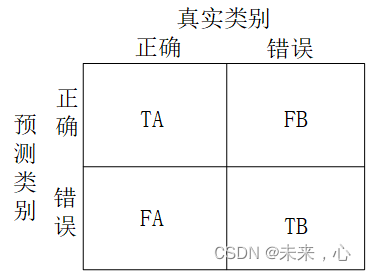
matrix The confusion matrix is ​​usually used to evaluate the quality of the training model. Here is a simple example of two classifications. There are categories A and B. The number of correct prediction results and A is recorded as TA, and the prediction results are correct and B The number of TB is recorded as TB, the wrong prediction and A is FA, and the wrong prediction and B is recorded as FB, so that a confusion matrix is ​​made. The display effect of the confusion matrix is ​​as follows, and the prediction results and quantities can be seen intuitively.

Below is the code for the confusion matrix

from sklearn.metrics import confusion_matrix
import seaborn as sns
import pandas as pd

# 定义一个绘制混淆矩阵图的函数
def plot_cm(labels, predictions):
    
    # 生成混淆矩阵
    conf_numpy = confusion_matrix(labels, predictions)
    # 将矩阵转化为 DataFrame
    conf_df = pd.DataFrame(conf_numpy, index=class_names ,columns=class_names)  
    
    plt.figure(figsize=(8,7))
    
    sns.heatmap(conf_df, annot=True, fmt="d", cmap="BuPu")
    
    plt.title('混淆矩阵',fontsize=15)
    plt.ylabel('真实值',fontsize=14)
    plt.xlabel('预测值',fontsize=14)
val_pre   = []
val_label = []

for images, labels in val_ds:#这里可以取部分验证数据（.take(1)）生成混淆矩阵
    for image, label in zip(images, labels):
        # 需要给图片增加一个维度
        img_array = tf.expand_dims(image, 0) 
        # 使用模型预测图片中的人物
        prediction = model.predict(img_array)

        val_pre.append(class_names[np.argmax(prediction)])
        val_label.append(class_names[label])
plot_cm(val_label, val_pre)

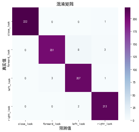
The following is the result of the confusion matrix of eye recognition

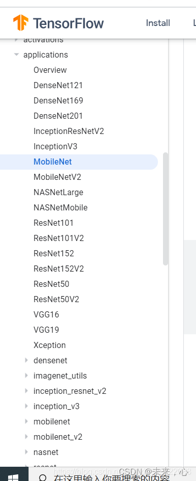
2. Commonly used network structure calling methods
Tensorflow comes with many levels of neural networks, which can be called through functions. The code below takes the VGG16 model call as an example.

model = tf.keras.applications.VGG16()
# 打印模型信息
model.summary()

The network models that can be called directly are listed below:

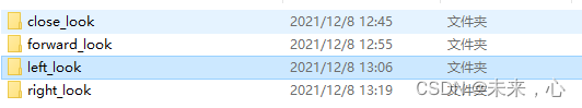
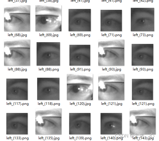
3. The eye data set is connected as follows:
Link: https://pan.baidu.com/s/12Waf0no8vKHhqUK8RzGmUA
Extraction code:
There are four files in n2v0:


4. The complete code is given at the end refer to

import matplotlib.pyplot as plt
# 支持中文
plt.rcParams['font.sans-serif'] = ['SimHei']  # 用来正常显示中文标签
plt.rcParams['axes.unicode_minus'] = False  # 用来正常显示负号

import os,PIL

# 设置随机种子尽可能使结果可以重现
import numpy as np
np.random.seed(1)

# 设置随机种子尽可能使结果可以重现
import tensorflow as tf
tf.random.set_seed(1)

import pathlib
data_dir = "H:\python_project\python辅助算法\data\\017_Eye_dataset"

data_dir = pathlib.Path(data_dir)
image_count = len(list(data_dir.glob('*/*')))

print("图片总数为：",image_count)
# 预处理数据
batch_size = 64
img_height = 224
img_width = 224
"""
关于image_dataset_from_directory()的详细介绍可以参考文章：https://mtyjkh.blog.csdn.net/article/details/117018789
"""
train_ds = tf.keras.preprocessing.image_dataset_from_directory(
    data_dir,
    validation_split=0.2,
    subset="training",
    seed=12,
    image_size=(img_height, img_width),
    batch_size=batch_size)
"""
关于image_dataset_from_directory()的详细介绍可以参考文章：https://mtyjkh.blog.csdn.net/article/details/117018789
"""
val_ds = tf.keras.preprocessing.image_dataset_from_directory(
    data_dir,
    validation_split=0.2,
    subset="validation",
    seed=12,
    image_size=(img_height, img_width),
    batch_size=batch_size)
class_names = train_ds.class_names
print(class_names)
# 配置数据集
AUTOTUNE = tf.data.AUTOTUNE

train_ds = train_ds.cache().shuffle(1000).prefetch(buffer_size=AUTOTUNE)
val_ds   = val_ds.cache().prefetch(buffer_size=AUTOTUNE)
# 调用模型
model = tf.keras.applications.VGG16()
# 打印模型信息
model.summary()
# 设置初始学习率
initial_learning_rate = 1e-4

lr_schedule = tf.keras.optimizers.schedules.ExponentialDecay(
        initial_learning_rate,
        decay_steps=20,      # 敲黑板！！！这里是指 steps，不是指epochs
        decay_rate=0.96,     # lr经过一次衰减就会变成 decay_rate*lr
        staircase=True)

# 将指数衰减学习率送入优化器
optimizer = tf.keras.optimizers.Adam(learning_rate=lr_schedule)
# 编译
model.compile(optimizer=optimizer,
              loss     ='sparse_categorical_crossentropy',
              metrics  =['accuracy'])
epochs = 10
# 训练
history = model.fit(
    train_ds,
    validation_data=val_ds,
    epochs=epochs
)
# 训练过程存储在history里面
acc = history.history['accuracy']
val_acc = history.history['val_accuracy']

loss = history.history['loss']
val_loss = history.history['val_loss']

epochs_range = range(epochs)
# 展示训练结果
plt.figure(figsize=(12, 4))
plt.subplot(1, 2, 1)

plt.plot(epochs_range, acc, label='Training Accuracy')
plt.plot(epochs_range, val_acc, label='Validation Accuracy')
plt.legend(loc='lower right')
plt.title('Training and Validation Accuracy')

plt.subplot(1, 2, 2)
plt.plot(epochs_range, loss, label='Training Loss')
plt.plot(epochs_range, val_loss, label='Validation Loss')
plt.legend(loc='upper right')
plt.title('Training and Validation Loss')
plt.show()

from sklearn.metrics import confusion_matrix
import seaborn as sns
import pandas as pd


# 定义一个绘制混淆矩阵图的函数
def plot_cm(labels, predictions):
    # 生成混淆矩阵
    conf_numpy = confusion_matrix(labels, predictions)
    # 将矩阵转化为 DataFrame
    conf_df = pd.DataFrame(conf_numpy, index=class_names, columns=class_names)

    plt.figure(figsize=(8, 7))

    sns.heatmap(conf_df, annot=True, fmt="d", cmap="BuPu")

    plt.title('混淆矩阵', fontsize=15)
    plt.ylabel('真实值', fontsize=14)
    plt.xlabel('预测值', fontsize=14)
val_pre   = []
val_label = []

for images, labels in val_ds:#这里可以取部分验证数据（.take(1)）生成混淆矩阵
    for image, label in zip(images, labels):
        # 需要给图片增加一个维度
        img_array = tf.expand_dims(image, 0)
        # 使用模型预测图片中的人物
        prediction = model.predict(img_array)

        val_pre.append(class_names[np.argmax(prediction)])
        val_label.append(class_names[label])
# 保存模型
model.save('model/17_model.h5')
# 加载模型
new_model = tf.keras.models.load_model('model/17_model.h5')
# 采用加载的模型（new_model）来看预测结果

plt.figure(figsize=(10, 5))  # 图形的宽为10高为5
plt.suptitle("预测结果展示")

for images, labels in val_ds.take(1):
    for i in range(8):
        ax = plt.subplot(2, 4, i + 1)

        # 显示图片
        plt.imshow(images[i].numpy().astype("uint8"))

        # 需要给图片增加一个维度
        img_array = tf.expand_dims(images[i], 0)

        # 使用模型预测图片中的人物
        predictions = new_model.predict(img_array)
        plt.title(class_names[np.argmax(predictions)])

        plt.axis("off")

The specific parameters of VGG16 are shown below. This model has many parameters, and there are many ways to optimize it.

Model: "vgg16"
_________________________________________________________________
Layer (type)                 Output Shape              Param #   
=================================================================
input_1 (InputLayer)         [(None, 224, 224, 3)]     0         
_________________________________________________________________
block1_conv1 (Conv2D)        (None, 224, 224, 64)      1792      
_________________________________________________________________
block1_conv2 (Conv2D)        (None, 224, 224, 64)      36928     
_________________________________________________________________
block1_pool (MaxPooling2D)   (None, 112, 112, 64)      0         
_________________________________________________________________
block2_conv1 (Conv2D)        (None, 112, 112, 128)     73856     
_________________________________________________________________
block2_conv2 (Conv2D)        (None, 112, 112, 128)     147584    
_________________________________________________________________
block2_pool (MaxPooling2D)   (None, 56, 56, 128)       0         
_________________________________________________________________
block3_conv1 (Conv2D)        (None, 56, 56, 256)       295168    
_________________________________________________________________
block3_conv2 (Conv2D)        (None, 56, 56, 256)       590080    
_________________________________________________________________
block3_conv3 (Conv2D)        (None, 56, 56, 256)       590080    
_________________________________________________________________
block3_pool (MaxPooling2D)   (None, 28, 28, 256)       0         
_________________________________________________________________
block4_conv1 (Conv2D)        (None, 28, 28, 512)       1180160   
_________________________________________________________________
block4_conv2 (Conv2D)        (None, 28, 28, 512)       2359808   
_________________________________________________________________
block4_conv3 (Conv2D)        (None, 28, 28, 512)       2359808   
_________________________________________________________________
block4_pool (MaxPooling2D)   (None, 14, 14, 512)       0         
_________________________________________________________________
block5_conv1 (Conv2D)        (None, 14, 14, 512)       2359808   
_________________________________________________________________
block5_conv2 (Conv2D)        (None, 14, 14, 512)       2359808   
_________________________________________________________________
block5_conv3 (Conv2D)        (None, 14, 14, 512)       2359808   
_________________________________________________________________
block5_pool (MaxPooling2D)   (None, 7, 7, 512)         0         
_________________________________________________________________
flatten (Flatten)            (None, 25088)             0         
_________________________________________________________________
fc1 (Dense)                  (None, 4096)              102764544 
_________________________________________________________________
fc2 (Dense)                  (None, 4096)              16781312  
_________________________________________________________________
predictions (Dense)          (None, 1000)              4097000   
=================================================================
Total params: 138,357,544
Trainable params: 138,357,544
Non-trainable params: 0

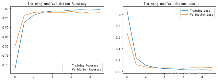
The following is the code display and graph of the training curve (training and verification):

acc = history.history['accuracy']
val_acc = history.history['val_accuracy']

loss = history.history['loss']
val_loss = history.history['val_loss']

epochs_range = range(epochs)

plt.figure(figsize=(12, 4))
plt.subplot(1, 2, 1)

plt.plot(epochs_range, acc, label='Training Accuracy')
plt.plot(epochs_range, val_acc, label='Validation Accuracy')
plt.legend(loc='lower right')
plt.title('Training and Validation Accuracy')

plt.subplot(1, 2, 2)
plt.plot(epochs_range, loss, label='Training Loss')
plt.plot(epochs_range, val_loss, label='Validation Loss')
plt.legend(loc='upper right')
plt.title('Training and Validation Loss')
plt.show()