average_precision_score() function----detailed calculation process and principle

Recently, when reproducing the paper, it was found that the author used the average_precision_score() function in the sklearn.metrics library to evaluate the classification model.

After reading many blog posts, I didn’t understand its principle and function, and I did n’t understand the official documents of sklean until I found this article Evaluating Object Detection Models Using Mean Average Precision (mAP) on Google. .

First, let me explain the calculation process:

1. Use the model to generate predictive scores .
2. Convert prediction scores to class labels by using a threshold .
3. Compute the confusion matrix .
4. Calculate the corresponding precision and recall .
5. Create a precision-recall curve .
6. Computes the average precision .

The following is divided into three stages to explain:

From Prediction Score to Class Label

In this section, we will quickly review how class labels are derived from prediction scores.

Suppose there are two categories, Positive and Negative, here are the true labels of 10 samples.

y_true = ["positive", "negative", "negative", "positive", "positive", "positive", "negative", "positive", "negative", "positive"]

When these samples are fed into the model, it returns the following prediction scores. Based on these scores, how do we classify the samples (i.e. assign each sample a class label)?

pred_scores = [0.7, 0.3, 0.5, 0.6, 0.55, 0.9, 0.4, 0.2, 0.4, 0.3]

To convert prediction scores to class labels , a threshold is used . When the score is equal to or higher than the threshold, the sample is classified into a class (usually positive class, 1). Otherwise, it is classified as something else (usually negative, 0).

The following code block converts the scores to class labels with a threshold of 0.5.

import numpy

pred_scores = [0.7, 0.3, 0.5, 0.6, 0.55, 0.9, 0.4, 0.2, 0.4, 0.3]
y_true = ["positive", "negative", "negative", "positive", "positive", "positive", "negative", "positive", "negative", "positive"]

threshold = 0.5
y_pred = ["positive" if score >= threshold else "negative" for score in pred_scores]
print(y_pred)

The converted tags are as follows:

['positive', 'negative', 'positive', 'positive', 'positive', 'positive', 'negative', 'negative', 'negative', 'negative']

Both the true and predicted labels are now available in the y_true and y_pred variables .

Based on these labels, the confusion matrix, precision and recall can be calculated . (You can read this blog post , which is very good, but the picture of the confusion matrix is ​​a little flawed)

r = numpy.flip(sklearn.metrics.confusion_matrix(y_true, y_pred))
print(r)

precision = sklearn.metrics.precision_score(y_true=y_true, y_pred=y_pred, pos_label="positive")
print(precision)

recall = sklearn.metrics.recall_score(y_true=y_true, y_pred=y_pred, pos_label="positive")
print(recall)

The result is

# Confusion Matrix (From Left to Right & Top to Bottom: True Positive, False Negative, False Positive, True Negative)
[[4 2]
 [1 3]]

# Precision = 4/(4+1)
0.8

# Recall = 4/(4+2)
0.6666666666666666

After a quick review of calculating precision and recall, we next discuss creating a precision-recall curve.

Precision-Recall Curve (Precision-Recall Curve)

Given the definitions of precision and recall, keep in mind that the higher the precision, the more confident the model can be in classifying a sample as positive. The higher the recall, the more positive examples the model correctly classifies as Positive.

When a model has high recall but low precision, the model correctly classifies most of the positive examples, but it has many false positives (i.e. classifies many negative examples as positive). When a model has high precision but low recall, the model is accurate in classifying samples as positive, but it may only classify some positive samples.
Note: I understand that in order for a model to truly achieve excellent results, both precision and recall should be high.

Because of the importance of precision and recall, a precision-recall curve can show the trade-off between precision and recall values ​​for different thresholds . This curve helps to choose the optimal threshold to maximize both metrics.

Creating a precision-recall curve requires a few inputs:

1. 真实标签。
2. 样本的预测分数。
3. 将预测分数转换为类别标签的一些阈值。

The next code block creates the y_true list to hold the true labels , the pred_scores list for the predicted scores , and finally the thresholds list for the different thresholds .

import numpy

y_true = ["positive", "negative", "negative", "positive", "positive", "positive", "negative", "positive", "negative", "positive", "positive", "positive", "positive", "negative", "negative", "negative"]

pred_scores = [0.7, 0.3, 0.5, 0.6, 0.55, 0.9, 0.4, 0.2, 0.4, 0.3, 0.7, 0.5, 0.8, 0.2, 0.3, 0.35]

thresholds = numpy.arange(start=0.2, stop=0.7, step=0.05)

This is the threshold saved in the threshold list. Since there are 10 thresholds, 10 precision and recall values ​​will be created.

[0.2, 
 0.25, 
 0.3, 
 0.35, 
 0.4, 
 0.45, 
 0.5, 
 0.55, 
 0.6, 
 0.65]

The next function called precision_recall_curve() receives the true label, prediction score and threshold . It returns two equal-length lists representing precision and recall values.

import sklearn.metrics

def precision_recall_curve(y_true, pred_scores, thresholds):
    precisions = []
    recalls = []
    
    for threshold in thresholds:
        y_pred = ["positive" if score >= threshold else "negative" for score in pred_scores]

        precision = sklearn.metrics.precision_score(y_true=y_true, y_pred=y_pred, pos_label="positive")
        recall = sklearn.metrics.recall_score(y_true=y_true, y_pred=y_pred, pos_label="positive")
        
        precisions.append(precision)
        recalls.append(recall)

    return precisions, recalls

The following code calls the precision_recall_curve() function after being passed three previously prepared lists. It returns a precision and recall list containing all values ​​for precision and recall respectively.

precisions, recalls = precision_recall_curve(y_true=y_true, 
                                             pred_scores=pred_scores,
                                             thresholds=thresholds)

The following are the return values ​​in the precision precision list

[0.5625,
 0.5714285714285714,
 0.5714285714285714,
 0.6363636363636364,
 0.7,
 0.875,
 0.875,
 1.0,
 1.0,
 1.0]

This is the list of values ​​in the recall list

[1.0,
 0.8888888888888888,
 0.8888888888888888,
 0.7777777777777778,
 0.7777777777777778,
 0.7777777777777778,
 0.7777777777777778,
 0.6666666666666666,
 0.5555555555555556,
 0.4444444444444444]

Given two lists of equal length, their values ​​can be plotted in a two-dimensional plot as follows

matplotlib.pyplot.plot(recalls, precisions, linewidth=4, color="red")
matplotlib.pyplot.xlabel("Recall", fontsize=12, fontweight='bold')
matplotlib.pyplot.ylabel("Precision", fontsize=12, fontweight='bold')
matplotlib.pyplot.title("Precision-Recall Curve", fontsize=15, fontweight="bold")
matplotlib.pyplot.show()

The precision-recall curve is shown in the figure below. Note that precision decreases as recall increases. The reason is that when the number of positive samples increases (high recall), the accuracy of correctly classifying each sample decreases (low precision). This is expected since the model is more likely to fail when there are many samples.

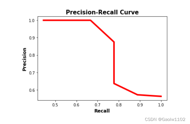
A precision-recall curve makes it easy to identify points where both precision and recall are high. According to the figure above, the best point is (recall, precision)=(0.778, 0.875).

Using the graph above to graphically determine the optimal values ​​for precision and recall might work because the curves are not complicated. A better approach is to use a metric called f1-score , which is calculated according to the next equation.

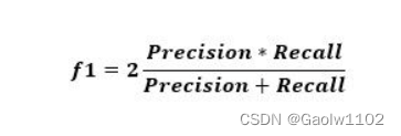
The f1 metric measures the balance between precision and recall. When the value of f1 is high, it means both precision and recall are high. A lower f1 score means a greater imbalance between precision and recall.

According to the previous example, f1 is calculated according to the following code. Based on the values ​​in the f1 list, the highest score is 0.82352941. It is the 6th element (ie index 5) in the list. The 6th element in the recall and precision lists are 0.778 and 0.875, respectively. The corresponding threshold is 0.45.

f1 = 2 * ((numpy.array(precisions) * numpy.array(recalls)) / (numpy.array(precisions) + numpy.array(recalls)))

The result is as follows

[0.72, 
 0.69565217, 
 0.69565217, 
 0.7,
 0.73684211,
 0.82352941, 
 0.82352941, 
 0.8, 
 0.71428571, 
 0.61538462]

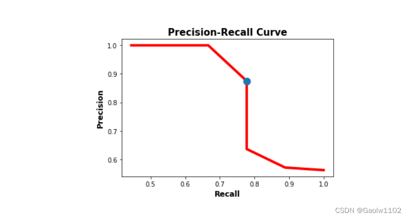
The image below shows in blue the location of the point corresponding to the best balance between recall and precision. In summary, the optimal threshold for balancing precision and recall is 0.45, where precision is 0.875 and recall is 0.778.

matplotlib.pyplot.plot(recalls, precisions, linewidth=4, color="red", zorder=0)
matplotlib.pyplot.scatter(recalls[5], precisions[5], zorder=1, linewidth=6)

matplotlib.pyplot.xlabel("Recall", fontsize=12, fontweight='bold')
matplotlib.pyplot.ylabel("Precision", fontsize=12, fontweight='bold')
matplotlib.pyplot.title("Precision-Recall Curve", fontsize=15, fontweight="bold")
matplotlib.pyplot.show()

After discussing the precision-recall curve, let's discuss how to calculate the average precision.

Average precision AP (Average Precision)

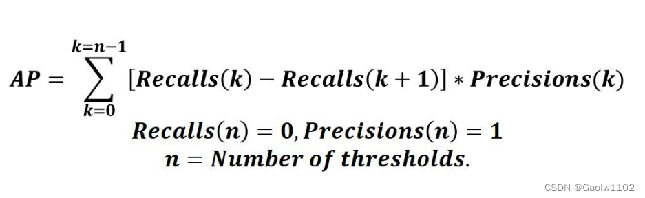
Average precision (AP) is a way to summarize the precision-recall curve into a single value representing the average of all precisions. AP is calculated according to the formula below. Use a loop to iterate over all precision/recalls, calculate the difference between the current recall and the next recall, and multiply by the current precision. In other words, Average-Precision is a weighted sum of precision for each threshold, where the weight is the difference in recall.

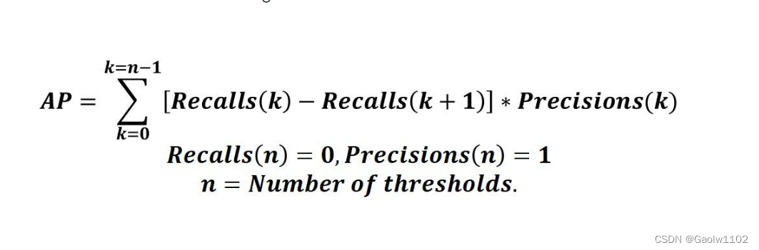
It is important to append 0 and 1 for recalls and precisions respectively. For example, if the recalls list is
$$0.8,0.6$$
appends 0 to it, which is
$$0.8,0.6,0.0$$
Similarly, append 1 to the precision list precsion,
$$0.8,0.2,1.0$$
Given that both recalls and precisions are NumPy arrays, the above equations are executed according to the following formula

AP = numpy.sum((recalls[:-1] - recalls[1:]) * precisions[:-1])

Below is the complete code to calculate AP

import numpy
import sklearn.metrics

def precision_recall_curve(y_true, pred_scores, thresholds):
    precisions = []
    recalls = []
    
    for threshold in thresholds:
        y_pred = ["positive" if score >= threshold else "negative" for score in pred_scores]

        precision = sklearn.metrics.precision_score(y_true=y_true, y_pred=y_pred, pos_label="positive")
        recall = sklearn.metrics.recall_score(y_true=y_true, y_pred=y_pred, pos_label="positive")
        
        precisions.append(precision)
        recalls.append(recall**

    return precisions, recalls

y_true = ["positive", "negative", "negative", "positive", "positive", "positive", "negative", "positive", "negative", "positive", "positive", "positive", "positive", "negative", "negative", "negative"]
pred_scores = [0.7, 0.3, 0.5, 0.6, 0.55, 0.9, 0.4, 0.2, 0.4, 0.3, 0.7, 0.5, 0.8, 0.2, 0.3, 0.35]
thresholds=numpy.arange(start=0.2, stop=0.7, step=0.05)

precisions, recalls = precision_recall_curve(y_true=y_true, 
                                             pred_scores=pred_scores, 
                                             thresholds=thresholds)

precisions.append(1)
recalls.append(0)

precisions = numpy.array(precisions)
recalls = numpy.array(recalls)

AP = numpy.sum((recalls[:-1] - recalls[1:]) * precisions[:-1])
print(AP)

Summarize

It should be noted that in the average_precision_score() function, some algorithmic adjustments have been made. Unlike the above, each prediction score will be used as a threshold to calculate the corresponding precision rate precision and recall rate recall. Finally , the Average-Precision formula is applied to the precisions and recalls lists with a length of len (prediction score) to obtain the final Average-Precision value.

Verify that the function is against the algorithm

Now from the official document of sklean, get the use case of this function, as follows ( official link )

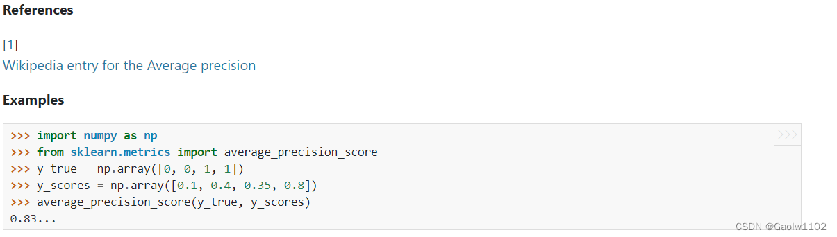
Now use the above algorithm to calculate

import sklearn.metrics

'''
计算在给定阈值thresholds下的所有精确率与召回率
'''
def precision_recall_curve(y_true, pred_scores, thresholds):
    precisions = []
    recalls = []
    
    for threshold in thresholds:
        y_pred = [1 if score >= threshold else 0 for score in pred_scores]                           # 对此处稍微做修改
        print('y_true is:', y_true)
        print('y_pred is:', y_pred)
        
        confusion_matrix = sklearn.metrics.confusion_matrix(y_true, y_pred)                          # 输出混淆矩阵 
        precision = sklearn.metrics.precision_score(y_true=y_true, y_pred=y_pred)                    # 输出精确率
        recall = sklearn.metrics.recall_score(y_true=y_true, y_pred=y_pred)                          # 输出召回率
        
        print('confusion_matrix is:', confusion_matrix)
        print('precision is:', precision)
        print('recall is:', recall)
        
        precisions.append(precision)
        recalls.append(recall)                                                                       # 追加精确率与召回率
        
        print('\n')
        
    return precisions, recalls

Calculate the precision and recall corresponding to each threshold , and finally get precisions, recalls

precisions, recalls = precision_recall_curve([0, 0, 1, 1], [0.1, 0.4, 0.35, 0.8], [0.1, 0.4, 0.35, 0.8])

'''
结果
y_true is: [0, 0, 1, 1]
y_pred is: [1, 1, 1, 1]
confusion_matrix is: [[0 2] [0 2]]
precision is: 0.5
recall is: 1.0


y_true is: [0, 0, 1, 1]
y_pred is: [0, 1, 0, 1]
confusion_matrix is: [[1 1] [1 1]]
precision is: 0.5
recall is: 0.5


y_true is: [0, 0, 1, 1]
y_pred is: [0, 1, 1, 1]
confusion_matrix is: [[1 1] [0 2]]
precision is: 0.6666666666666666
recall is: 1.0


y_true is: [0, 0, 1, 1]
y_pred is: [0, 0, 0, 1]
confusion_matrix is: [[2 0] [1 1]]
precision is: 1.0
recall is: 0.5
'''

Add 1, 0 to the precisions list and the recalls list respectively , and output the precisions list and the recalls list

precisions.append(1), recalls.append(0)
precisions, recalls
'''
结果
([0.5, 0.5, 0.6666666666666666, 1.0, 1], [1.0, 0.5, 1.0, 0.5, 0])
'''

Substituting into the Average-Precision formula, we get

avg_precision = 0                                         # 初始化结果为0

# 不断加权求和
for i in range(len(precisions)-1):
    avg_precision += precisions[i] * (recalls[i] - recalls[i+1])

print('avg_precision is:', avg_precision)                 # 输出结果 

The output is

avg_precision is: 0.8333333333333333

It can be seen that the execution result of the sklearn.matrics.average_precision_score() algorithm is consistent, so it is correct.

epilogue

The above content is calculated after carefully checking the data, and there may be some inaccuracies. If you have any objections, please leave a comment!