1. Brief introduction of the paper
1. First author: Xiaofeng Wang
2. Year of publication: 2022
3. Published journal: ECCV
4. Keywords: MVS, 3D reconstruction, Transformer, epipolar geometry
5. Exploration motivation: Fusion of multi-view cost bodies is critical. Existing methods are inefficient, introduce too many additional parameters, and only focus on the information of image local correlation, ignoring the association of depth information.
存在问题:Fusing source volumes is an essential step in the whole pipeline and many MVS approaches put efforts into it. The core of the fusing step is to explore correlations between multi-view images. MVSNet follows the philosophy that various images contribute equally to the 3D cost volume, and utilizes variance operation to fuse different source volumes. However, such fusing method ignores various illumination and visibility conditions of different views.
一些解决办法:”To alleviate this problem, Transmvsnet、Patchmatchnet、CDS-MVSNet enrich 2D feature semnatics via Deformable Convolution Network (DCN) and PVA-MVSNet、Vis-MVSNet leverage extra networks to learn per-pixel weights as a guidance for fusing multi-view features.
这些办法的缺点:However, these methods introduce onerous network parameters and restrict efficiency. Besides, they only concentrate on 2D local similarities as a criteria for correlating multiple views, neglecting depth-wise 3D associations, which could lead to inconsistency in 3D space.
6. Working goal: Through Transformer, learn 3D relationship from the data itself without introducing additional learning parameters. Explore an efficient approach to modeling 3D spatially associative fused source-view volumes.
we explore an efficient approach to model 3D spatial associations for fusing source volumes. Our intuition is to learn 3D relations from data itself, without introducing extra learning parameters. Recent success in attention mechanism prompts that Transformer is appropriate for modeling 3D associations. The key advantage of Transformer is it leverages cross-attention to build data-dependent correlations, introducing minimal learnable parameters. Besides, compared with CNN, Transformer has expanded receptive field, which is more adept at constructing long-range 3D relations.
7. Core idea:
- We propose a novel end-to-end Transformer-based method for multi-view stereo, named MVSTER. It leverages the proposed epipolar Transformer to efficiently learn 3D associations along epipolar line.
- An auxiliary monocular depth estimator is utilized to guide the query feature to learn depth discriminative information during training, which enhances feature semantics yet brings no efficiency compromises.
- We formulate depth estimation as a depth-aware classification problem and solve it with the entropy-regularized optimal transport, which produces finer depth estimations propagated in the cascade structure.
8. Experimental results:
Compared with MVSNet and CasMVSNet, our method reduces 88% and 73% relative depth hypotheses, making 80% and 51% relative reduction in running time, yet obtaining 34% and 14% relative improvements on the DTU benchmark, respectively. Besides, our method ranks first among all published works on Tanks&Temples-Advanced.
9. Paper & code download:
https://arxiv.org/pdf/2204.07346v1.pdf
https://github.com/JeffWang987/MVSTER
2. Implementation process
1. Overview of MVSTER
The MVSTER network structure is shown in the figure. Given a reference image and its corresponding source image, a feature pyramid network is first utilized to extract 2D multi-scale features. The source image features are then transformed to the reference camera frustum, and the source volume is constructed by differentiable homography. Subsequently, the Jiji Transformer is used to aggregate the source body and generate a cost body, and the auxiliary branch performs monocular depth estimation to enhance the context. The volume is regularized by a lightweight 3D CNN for depth estimation pipeline further built in a cascaded structure, propagating the depth map in a coarse-to-fine manner . To reduce false depth assumptions during depth propagation, depth estimation is formulated as a depth-aware classification problem and optimized using an optimal transfer. Finally, the network loss is given .

2. 2D Encoder and 3D Homography
A FPN - like network is applied to extract multi-scale 2D features of a reference image and its neighboring source images . fpn, where the image is downscaled M times to build a deep feature Fk . Scale k = 0 represents the original size of the image. N−1 source volumes {Vi}N−1 ∈ H×W×C×D are obtained by homography change , where D is the total number of assumed depths.
3. Polar Transformer
Polar Transformer aggregates source volumes from different views. The epipolar Transformer uses the reference feature as a query to match the source feature (key) along the epipolar line , thereby enhancing the corresponding depth (value). Specifically, reference queries are enriched by an auxiliary task of monocular depth estimation. Subsequently, cross-attention computes the association between query and source volumes under epipolar constraints, generating attention guides to aggregate feature volumes from different views. Then, the aggregated features are regularized by a lightweight 3D CNN. In the following, we first give the details of the query construction, and then elaborate on the epipolar Transformer-guided feature aggregation. Finally, a lightweight regularization strategy is given.
Query construction. As mentioned before, we treat the reference feature as a query for the epipolar transformer. However, features extracted by shallow 2D CNNs are less discriminative in non-Lambertian and low-textured regions. To solve this problem, some methods utilize costly DCN or ASPP to enrich features. In contrast, this paper proposes a more effective way to augment queries: building an auxiliary monocular depth estimation branch to regularize queries and learn deep discriminative features. A generic decoder used in the monocular depth estimation task is applied in the auxiliary branch. Given the multi-scale reference features extracted by FPN, the low-resolution feature maps are expanded by interpolation and concatenated with subsequent scale features. The aggregated feature maps are fed into the regression head for monocular depth estimation:

Where Φ(⋅) is the monocular depth decoder, I(⋅) is the interpolation function, and [⋅,⋅] represents the connection operation. Subsequently, monocular depth estimation is queried for different scales. It is worth noting that this auxiliary branch is only used in the training phase to guide the network to learn depth-aware features.
Epipolar Transformer guided aggregation. The Pipeline, shown in Figure 2(a), aims to construct a 3D association of query features. However, the 3D spatial information in the depth direction is not explicitly conveyed by the 2D query feature map, so we first recover the depth information by homography warping. Project the assumed depth position of the query feature pr onto the epipolar line of the source image to obtain the source body feature psi,j, which is the key of the epipolar line transformer. Therefore, key features along epipolar lines are used to construct deep 3D associations of query features, which is achieved by the cross-attention operation:

where vi ∈ C×D is {psi,j} superimposed calculation along the depth dimension, te is the temperature parameter, and wi is the attention related to the query and the key. An example of a real image is visualized in Figure 2(b) , where attention is focused on the best matching location on the epipolar line.

(a) Epipolar Transformer aggregation. The depth information of the reference features is recovered using the homography variation, and then the 3D association between the query and the source volume is computed with cross-attention under extreme constraints, and attention guides are generated to aggregate feature volumes from different viewpoints. (b) Visualization of cross-attention scores on the DTU dataset , where the opacity of points on the epipolar line represents the attention score.
The calculated attention wi between query and keys is used to aggregate values. For Transformer's value design, group correlation is used to measure the visual similarity between reference features and source volumes in an efficient manner :

<·,·> is the inner product. Stacking along the channel dimension yields si∈G×D, which is the value of the Transformer. Finally, the value is aggregated by the epipolar attention score wi to determine the final cost body:

In summary, for the proposed epipolar Transformer, a separable monocular depth estimation branch is first utilized to enhance depth-discriminative 2D semantics, and then cross-attention between queries and keys is used to construct depth-wise 3D associations. Finally, combining 2D and 3D information is used as guidance for aggregating different views. The Epipolar Transformer is designed as an efficient aggregation module, where no learnable parameters are introduced, and the Epipolar Transformer only learns data-dependent associations.
Lightweight regularization. The original cost volume is susceptible to noise pollution due to non-Lambertian surfaces or object occlusions . To smooth the final depth map, a 3D CNN is used to regularize the cost volume . Considering that the 3D association has been embedded into the cost volume, deep feature encoding is omitted in 3D CNN, which makes it more efficient. Specifically, the convolution kernel size is reduced from 3 × 3 × 3 to 3 × 3 × 1, and the cost volume is only aggregated along the feature width and height. Regularized probability volume P ∈ H × W × D. It is ideal for per-pixel depth confidence prediction and is used for depth estimation in a cascaded structure.
4. Cascade depth map propagation
MVSTER sets up a four-stage pipeline, where the input resolutions of the four stages are H × W × 64 , H/2×W/2×32, H/4 × W/4 ×16, H/8 × W/ 8×8 . The first stage uses depth inverse sampling to initialize the depth hypothesis, which is equivalent to equidistant sampling of pixel space. In order to achieve the coarse-to-fine depth map propagation, the depth hypothesis of each stage is centered on the depth prediction of the previous stage, and Dk hypotheses are uniformly generated in the assumed depth range .
5. Loss
While the cascaded structure benefits from a coarse-to-fine pipeline, it is difficult to recover from errors introduced by previous stages. To alleviate this problem, a simple approach is to generate a finer depth map at each stage, especially to avoid predicting depths far from the ground truth. However, previous methods simply treat depth estimation as a multi-class classification problem, treating each hypothetical depth equally without considering the distance relationship among them. For example, in the figure below, the leftmost sub-number is a true depth, case 1 and case 2 are two predicted depth distributions, and their cross-entropy loss is the same, indicating that the cross-entropy loss does not know the difference between each assumed depth relative distance. However, the depth prediction of case 1 is beyond the effective range and cannot be propagated to the next stage normally.

In this paper, depth prediction is formulated as a depth-aware classification problem, which emphasizes the penalty of predicted depth versus ground-truth distance. Specifically, the off-the-shelf Wasserstein distance is used to measure the distance between the predicted distribution Pi∈D and the true distribution Pθ,i∈D:

Among them, inf represents the extreme value, Π(Pi, Pθ , i) is the set of all possible distributions with marginal distributions Pi and Pθ , i . Such a formulation is inspired by the optimal transport problem, which computes the minimum work Pθi to transport Pi to , which can be solved differentially by the sunken angle algorithm .
In summary, the loss function consists of two parts : the Wasserstein loss that measures the distance between the predicted depth distribution and the true value, and the L1 loss that optimizes monocular depth estimation :

6. Experiment
6.1. Datasets
DTU, Tanks&Temples, BlendedMVS,ETH3D
6.2. Implementation Details
Assume that the depth number {Dk} is set to 8, 8, 4, 4 for each segment. The group correlation {Gk} is set to 8,8,4,4. We use the PyTorch [21] implementation, training on 4 NVIDIA RTX 3090 GPUs with a batch size of 2 on each GPU. Use the AdamW optimizer [19].
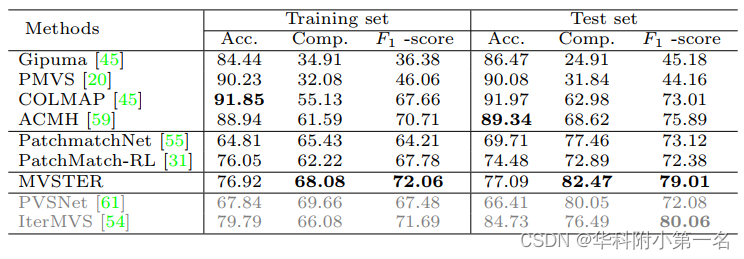
6.3. Comparison with advanced technologies

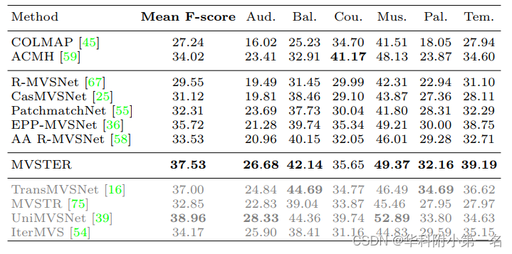
ETH3D