foreword
In the past, many basic models of recommendation system + deep learning have been obtained. From this article, we have also entered the chapter of attention mechanism. At the beginning of AFM, everyone is no longer limited to the problem of pairwise interaction of features, but began to explore some new structures. The word "Attention Mechanism" is not a new thing now, it comes from the natural choice of human beings to pay attention to the habit, the most typical example is that when we observe some objects or browse the web, we will not focus on the entire object or page, but will choose Continually pay attention to some specific areas, ignore some areas, and tend to focus on some conspicuous places. If the influence of the attention mechanism on the prediction results is considered in the modeling process, the effect will often be better. In recent years, the attention mechanism has shined in various fields, such as NLP, CV, etc. Since 2017, the recommendation field has also begun to try to add the attention mechanism to the model, such as today's AFM.
Today, I will introduce some appetizers AFM of recommendation system + attention mechanism. First, let’s take a look at the knowledge system that has been sorted out by Mr. Wang Zhe’s " Deep Learning Recommendation System".

1. AFM model
The AFM (Attentional Factorization Machines) model is also a model proposed by researchers from Zhejiang University and the National University of Singapore in 2017. The AFM model is actually an evolutionary version of the NFM model explained above. This model is very similar in structure to the NFM model. An extension of the NFM model. In NFM, the feature embedding vectors of different feature domains are crossed through the feature cross pooling layer, and the cross feature vectors are "summed", and then followed by a DNN network, but the addition in NFM And pooling, it is equivalent to "treating all cross-features equally", without considering the degree of influence of different features on the results, the author believes that this may affect the final prediction effect, because not all interactive features can play a role in the final prediction effect. Interaction features that are not useful can create noise. In other words, increase the features that are important to the prediction results and suppress the noise features.
For example, if the application scenario is to predict the possibility of whether a male user will purchase a keyboard, then the intersection feature of "gender = male and the purchase history includes a mouse" is likely to be higher than "gender = male and user age = 30 "This crossover feature is important. So it is not very reasonable for NFM to perform indiscriminate sum pooling on all second-order cross features. Therefore, it is very reasonable to introduce the attention mechanism!
First look at the model architecture of AFM:
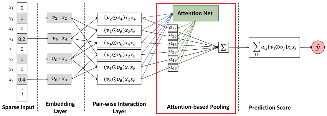
It can be seen that there is no DNN module in this model, but the second-order cross feature pooling layer of NFM is preserved.
2. Second-order cross-pooling layer
The second-order cross-pooling layer here is exactly the same as the NFM mentioned earlier, so I won't describe it here. But what needs to be noted here is that the addition of Attention does not just give a weight to a certain two-dimensional cross-feature. In this way, it is impossible to assign weights to cross-features that do not appear in the training data. So in the above figure, you can also see that Attention is given in the form of a Net. That is, an MLP is used to parameterize the attention score.
The structure of the attention network is a simple single fully connected layer plus softmax output layer structure, the mathematical expression is as follows:
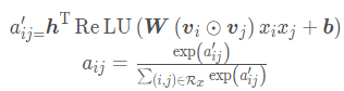
The learned model parameters are the weight matrix W and bias vector b from the feature intersection layer to the fully connected layer of the attention network, and the weight vector h from the fully connected layer to the softmax output layer. The dimensions of these three are , , ,
where
t tt represents the number of units in the hidden layer of the attention network.
It indicates the importance of each interaction feature. After passing softmax, this is a value between 0-1. The attention network participates in the backpropagation process together with the whole model to get the final weight parameters.
The output of the attention-based pooling layer is a k-dimensional vector, which is an aggregation effect after all feature interaction vectors are distinguished according to the degree of importance, and then we map it to the final prediction score. So the overall formula of AFM is as follows:

Regarding the learning part of the model, of course it comes according to different tasks. This model can also be used for both regression tasks and classification tasks. Compared with NFM, the DNN network is not used to learn high-level interactions at present. This is tentative For the author's future research work. That's all about the work of AFM, and it is also very simple (by no means I am in the water article~).
3, pytorch reproduction
class Dnn(nn.Module):
    def __init__(self, hidden_units, dropout=0.):
        """
        hidden_units: 列表, 每个元素表示每一层的神经单元个数, 比如[256, 128, 64], 两层网络, 第一层神经单元128, 第二层64, 第一个维度是输入维度
        dropout = 0.
        """
        super(Dnn, self).__init__()

        self.dnn_network = nn.ModuleList([nn.Linear(layer[0], layer[1]) for layer in list(zip(hidden_units[:-1], hidden_units[1:]))])
        self.dropout = nn.Dropout(dropout)

    def forward(self, x):
        for linear in self.dnn_network:
            x = linear(x)
            x = F.relu(x)
        x = self.dropout(x)
        return x

class Attention_layer(nn.Module):
    def __init__(self, att_units):
        """
        :param att_units: [embed_dim, att_vector]
        """
        super(Attention_layer, self).__init__()

        self.att_w = nn.Linear(att_units[0], att_units[1])
        self.att_dense = nn.Linear(att_units[1], 1)

    def forward(self, bi_interaction):     # bi_interaction (None, (field_num*(field_num-1)_/2, embed_dim)
        a = self.att_w(bi_interaction)    # (None, (field_num*(field_num-1)_/2, embed_dim)
        a = F.relu(a)             # (None, (field_num*(field_num-1)_/2, embed_dim)
        att_scores = self.att_dense(a)  # (None, (field_num*(field_num-1)_/2, 1)
        att_weight = F.softmax(att_scores, dim=1)  #  (None, (field_num*(field_num-1)_/2, 1)

        att_out = torch.sum(att_weight * bi_interaction, dim=1)   # (None, embed_dim)
        return att_out


class AFM(nn.Module):
    def __init__(self, feature_columns, mode, hidden_units, att_vector=8, dropout=0.5, useDNN=False):
        """
        AFM:
        :param feature_columns: 特征信息, 这个传入的是fea_cols array[0] dense_info  array[1] sparse_info
        :param mode: A string, 三种模式, 'max': max pooling, 'avg': average pooling 'att', Attention
        :param att_vector: 注意力网络的隐藏层单元个数
        :param hidden_units: DNN网络的隐藏单元个数, 一个列表的形式, 列表的长度代表层数, 每个元素代表每一层神经元个数, lambda文里面没加
        :param dropout: Dropout比率
        :param useDNN: 默认不使用DNN网络
        """
        super(AFM, self).__init__()
        self.dense_feature_cols, self.sparse_feature_cols = feature_columns
        self.mode = mode
        self.useDNN = useDNN

        # embedding
        self.embed_layers = nn.ModuleDict({
            'embed_' + str(i): nn.Embedding(num_embeddings=feat['feat_num'], embedding_dim=feat['embed_dim'])
            for i, feat in enumerate(self.sparse_feature_cols)
        })

        # 如果是注意机制的话,这里需要加一个注意力网络
        if self.mode == 'att':
            self.attention = Attention_layer([self.sparse_feature_cols[0]['embed_dim'], att_vector])

        # 如果使用DNN的话, 这里需要初始化DNN网络
        if self.useDNN:
            # 这里要注意Pytorch的linear和tf的dense的不同之处, 前者的linear需要输入特征和输出特征维度, 而传入的hidden_units的第一个是第一层隐藏的神经单元个数,这里需要加个输入维度
            self.fea_num = len(self.dense_feature_cols) + self.sparse_feature_cols[0]['embed_dim']
            hidden_units.insert(0, self.fea_num)

            self.bn = nn.BatchNorm1d(self.fea_num)
            self.dnn_network = Dnn(hidden_units, dropout)
            self.nn_final_linear = nn.Linear(hidden_units[-1], 1)
        else:
            self.fea_num = len(self.dense_feature_cols) + self.sparse_feature_cols[0]['embed_dim']
            self.nn_final_linear = nn.Linear(self.fea_num, 1)

    def forward(self, x):
        dense_inputs, sparse_inputs = x[:, :len(self.dense_feature_cols)], x[:, len(self.dense_feature_cols):]
        sparse_inputs = sparse_inputs.long()       # 转成long类型才能作为nn.embedding的输入
        sparse_embeds = [self.embed_layers['embed_'+str(i)](sparse_inputs[:, i]) for i in range(sparse_inputs.shape[1])]
        sparse_embeds = torch.stack(sparse_embeds)     # embedding堆起来, (field_dim, None, embed_dim)
        sparse_embeds = sparse_embeds.permute((1, 0, 2))
        # 这里得到embedding向量之后 sparse_embeds(None, field_num, embed_dim)
        # 下面进行两两交叉, 注意这时候不能加和了,也就是NFM的那个计算公式不能用, 这里两两交叉的结果要进入Attention
        # 两两交叉enbedding之后的结果是一个(None, (field_num*field_num-1)/2, embed_dim)
        # 这里实现的时候采用一个技巧就是组合
        #比如fild_num有4个的话,那么组合embeding就是[0,1] [0,2],[0,3],[1,2],[1,3],[2,3]位置的embedding乘积操作
        first = []
        second = []
        for f, s in itertools.combinations(range(sparse_embeds.shape[1]), 2):
            first.append(f)
            second.append(s)
        # 取出first位置的embedding  假设field是3的话,就是[0, 0, 0, 1, 1, 2]位置的embedding
        p = sparse_embeds[:, first, :]     # (None, (field_num*(field_num-1)_/2, embed_dim)
        q = sparse_embeds[:, second, :]   # (None, (field_num*(field_num-1)_/2, embed_dim)
        bi_interaction = p * q    # (None, (field_num*(field_num-1)_/2, embed_dim)

        if self.mode == 'max':
            att_out = torch.sum(bi_interaction, dim=1)  #  (None, embed_dim)
        elif self.mode == 'avg':
            att_out = torch.mean(bi_interaction, dim=1)  # (None, embed_dim)
        else:
            # 注意力网络
            att_out = self.attention(bi_interaction)  # (None, embed_dim)

        # 把离散特征和连续特征进行拼接
        x = torch.cat([att_out, dense_inputs], dim=-1)

        if not self.useDNN:
            outputs = F.sigmoid(self.nn_final_linear(x))
        else:
            # BatchNormalization
            x = self.bn(x)
            # deep
            dnn_outputs = self.nn_final_linear(self.dnn_network(x))
            outputs = F.sigmoid(dnn_outputs)

        return outputs