Detailed explanation of backpropagation and gradient descent in neural networks

Abstract: Backpropagation refers to the method of computing the gradient of the parameters of a neural network.

This article is shared from Huawei Cloud Community " Detailed Explanation of Backpropagation and Gradient Descent ", author: Embedded Vision.

1. Forward propagation and back propagation

1.1, neural network training process

The neural network training process is:

First "guess" a result (model forward propagation process) through random parameters, which is called prediction result a here ;
Then calculate the gap between a and the sample label value y (that is, the calculation process of the loss function);
Then update the neuron parameters through the backpropagation algorithm, and try again with the new parameters. This time it is not a "guess", but approaching the correct direction with a basis. After all, the adjustment of the parameters is strategic (based on the gradient drop strategy).

The above steps are repeated many times until there is almost no difference between the predicted result and the real result, that is, |a−y|→0, then the training ends.

1.2, forward propagation

Forward propagation (or forward pass) refers to: computing and storing the results of each layer in the neural network in order (from the input layer to the output layer).

In order to better understand the calculation process of forward propagation, we can draw the forward propagation calculation diagram of the network according to the network structure. The following figure is an example of a simple network and the corresponding calculation graph:

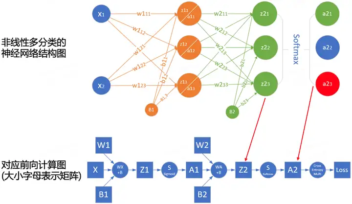
The squares represent variables, and the circles represent operators. The direction of data flow is calculated sequentially from left to right.

1.3, backpropagation

Backpropagation (backward propagation, referred to as BP) refers to the method of calculating the gradient of neural network parameters . Its principle is based on the chain rule in calculus , traverses the network from the output layer to the input layer in reverse order, and calculates the gradient of each intermediate variable and parameter in turn.

The automatic calculation of gradients (automatic differentiation) greatly simplifies the implementation of deep learning algorithms.

Note that the backpropagation algorithm will reuse the intermediate values stored in the forward propagation to avoid repeated calculations. Therefore, the intermediate results of the forward propagation need to be preserved, which will also cause the model training to require more memory than pure prediction ( video memory). At the same time, the memory (video memory) size occupied by these intermediate results is proportional to the number of network layers and the batch size (batch_size), so using a large batch_size to train a deeper network is more likely to cause out of memory (out of memory) errors!

1.4, Summary

Forward propagation computes and stores intermediate variables sequentially in the computational graph defined by the neural network, from the input layer to the output layer.
Backpropagation computes and stores the gradients of the intermediate variables and parameters of the neural network in reverse order (from the output layer to the input layer).
When training a neural network, after initializing the model parameters, we alternately use forward propagation and backpropagation, based on the gradient calculated by backpropagation, combined with the stochastic gradient descent optimization algorithm (or other optimization algorithms such as Adam) to update the model parameters .
Deep learning model training requires more memory than prediction.

Second, gradient descent

2.1, Optimization in Deep Learning

Most deep learning algorithms involve some form of optimization. The purpose of the optimizer is to update the network weight parameters so that we smoothly reach the minimum point of the loss value in the loss surface .

There are many challenges in deep learning optimization. Some of the most annoying are local minima, saddle points, and vanishing gradients.

Local minimum : For any objective function f(x), if the corresponding value of f(x) at x is less than the value of f(x) at any other point near x , then f(x) may be local min. If the value of f(x) at x is the minimum of the objective function over the entire domain, then f ( x ) is a global minimum.
Saddle point : Refers to any position where all gradients of a function vanish but is neither a global minimum nor a local minimum.
Vanishing gradient: For some reasons, the gradient of the objective function f is close to zero (that is, the gradient disappearance problem), which is one of the reasons why it is quite difficult to train the deep learning model before introducing the ReLU activation function and ResNet.

In deep learning, most of the objective functions are complex and there is no analytical solution, therefore, we need to use numerical optimization algorithms, and the optimization algorithms in this paper: SGD and Adam belong to this category.

2.2, how to understand the gradient descent method

The gradient descent (GD) algorithm is the most common optimizer in neural network model training. Although gradient descent is rarely used directly in deep learning, understanding it is fundamental to understanding stochastic gradient descent and mini-batch stochastic gradient descent algorithms.

Most articles use the example of "a person is trapped on a mountain and needs to quickly descend to the bottom of the valley" to understand the gradient descent method, but this is not entirely accurate. In nature, the best example of gradient descent is the process of spring water going downhill:

Water is affected by gravity and will flow in the steepest direction at the current position , sometimes forming a waterfall ( the opposite direction of the gradient is the direction in which the function value drops the fastest );
The path of water flowing down the mountain is not unique. At the same location, there may be multiple locations with the same steepness, which causes diversion (multiple solutions can be obtained);
Encountering potholes, lakes may form, and the downhill process will be terminated (the global optimal solution cannot be obtained, but a local optimal solution).

Examples refer to AI-EDU: Gradient Descent.

2.3, the principle of gradient descent

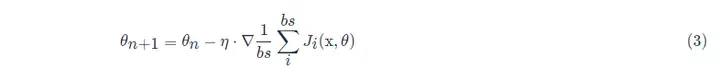
The mathematical formula for gradient descent:

in:

θn+1: the next value (updated value of the parameters in the neural network);
θn: current value (current parameter value);
−: Minus sign, the reverse of the gradient (the reverse direction of the gradient is the direction in which the function value decreases the fastest);
η: learning rate or step size, control the distance traveled by each step, not too fast to avoid missing the best scenic spots, not too slow to avoid too long time (hyperparameters that need to be manually adjusted);
∇: Gradient, the fastest rising point of the current position of the function (the gradient vector points uphill, and the negative gradient vector points downhill);
J(θ): function (objective function waiting to be optimized).

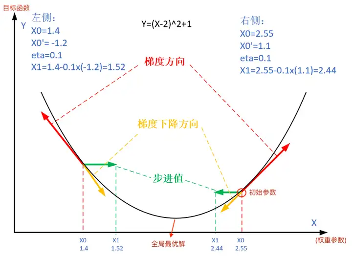
The figure below shows the steps of the gradient descent method. The purpose of gradient descent is to make the x value approach the extreme point.

Since it is bivariate, the iterative process of gradient descent needs to be explained with a three-dimensional plot. Table 2 visualizes the gradient descent process in 3D space.

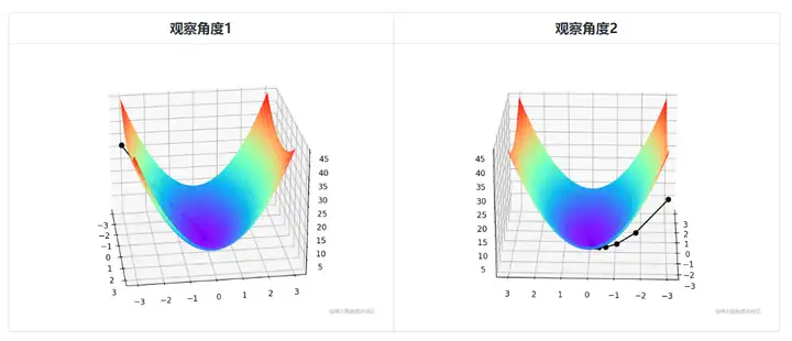
The faint black line in the middle of the figure represents the process of gradient descent, from the red highland all the way down the slope until the blue depression.

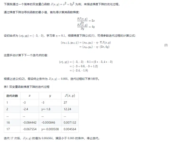
The gradient descent optimization process and visualization code of the bivariate convex function J(x,y)=x2+2y2 are as follows:

import numpy as np
import matplotlib.pyplot as plt
from mpl_toolkits.mplot3d import Axes3D
def target_function(x,y):
    J = pow(x, 2) + 2*pow(y, 2)
 return J
def derivative_function(theta):
    x = theta[0]
    y = theta[1]
 return np.array([2*x, 4*y])
def show_3d_surface(x, y, z):
    fig = plt.figure()
    ax = Axes3D(fig)
    u = np.linspace(-3, 3, 100)
    v = np.linspace(-3, 3, 100)
    X, Y = np.meshgrid(u, v)
    R = np.zeros((len(u), len(v)))
 for i in range(len(u)):
 for j in range(len(v)):
 R[i, j] = pow(X[i, j], 2)+ 4*pow(Y[i, j], 2)
 ax.plot_surface(X, Y, R, cmap='rainbow')
 plt.plot(x, y, z, c='black', linewidth=1.5,  marker='o', linestyle='solid')
 plt.show()
if __name__ == '__main__':
    theta = np.array([-3, -3]) # 输入为双变量
    eta = 0.1 # 学习率
    error = 5e-3 # 迭代终止条件，目标函数值 < error
    X = []
    Y = []
    Z = []
 for i in range(50):
 print(theta)
        x = theta[0]
        y = theta[1]
        z = target_function(x,y)
 X.append(x)
 Y.append(y)
 Z.append(z)
 print("%d: x=%f, y=%f, z=%f" % (i,x,y,z))
 d_theta = derivative_function(theta)
 print("    ", d_theta)
        theta = theta - eta * d_theta
 if z < error:
 break
    show_3d_surface(X,Y,Z)

Notice! To sum up, different step sizes η will lead to different changes in the value of the optimized function J as the number of iterations increases:

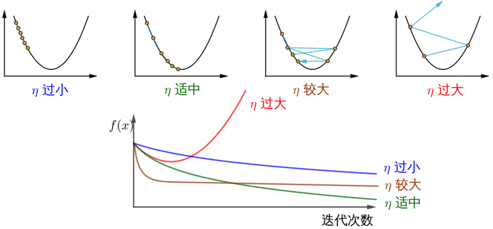
How does the image source understand the gradient descent method? .

Three, stochastic gradient descent and small batch stochastic gradient descent

3.1, stochastic gradient descent

In deep learning, the objective function is usually the average of the loss function for each sample in the training dataset. If gradient descent is used, the computational cost per independent variable iteration is O(n), which grows linearly with n (number of samples). Therefore, when the training dataset is large, the computational cost of gradient descent per iteration will be high.

Stochastic Gradient Descent (SGD) reduces the computational cost at each iteration. In each iteration of stochastic gradient descent, we uniformly sample a data sample at random at an index i, where i ∈ 1,...,n, and compute the gradient ∇J(θ) to update the weight parameter θ:

The computational cost per iteration drops from O(n) for gradient descent to a constant O(1). Also, it's worth emphasizing that the stochastic gradient ∇J(θ) is an unbiased estimate of the full gradient ∇J(θ).

An unbiased estimate is an unbiased inference when a sample statistic is used to estimate a population parameter.

In practical applications, the stochastic gradient descent SGD method must be used in combination with the dynamic learning rate method, otherwise the combination of fixed learning rate + SGD will make the model convergence process more complicated.

3.2, mini-batch stochastic gradient descent

The gradient descent (GD) and stochastic gradient descent (SGD) methods mentioned above are too extreme, either using the full data set to calculate the gradient and update the parameters, or only process one training sample at a time to update the parameters. In actual projects, a compromise will be made between the two, that is, minibatch gradient descent. Using minibatch gradient descent can also improve computational efficiency.

All sample data elements in the mini-batch are randomly drawn from the training set, and the number of samples is batch_size (abbreviated as bs)

In addition, the SGD optimization algorithm used in general projects will use small batch stochastic gradient descent by default, that is, batch_size > 1, unless the graphics card memory is insufficient, batch_size = 1 will be set.

References

How to understand the gradient descent method?
AI-EDU: Gradient Descent
"Hands-on Deep Learning Chapter 11 - Optimization Algorithms"

Click to follow and learn about Huawei Cloud's fresh technologies for the first time~