Original article, reprint please indicate that it is from "Old Cake Explains Neural Network" : bp.bbbdata.com

About "Old Cake Explains Neural Network":

This website explains the knowledge, principles and codes of neural networks in a structured way.

Reproduce the algorithm of matlab neural network toolbox, it is a good assistant for learning neural network.

Table of contents

1. Introduction to BP model

01. BP structure and bionic ideas

02. Commonly used BP structure

03. Mathematical structure of BP (expression)

2. Gradient descent method to solve BP neural network

01. Problem

02. Modeling ideas

03. Code implementation

04. Running results

05. Check the effect of the model

The first part of this article first introduces the model structure and mathematical expressions of the BP neural network.

The second part introduces the specific examples and codes of solving the BP neural network with the gradient descent method (without relying on any third-party packages).

The typesetting is messy and will not be adjusted anymore. If you need it, you can directly check it on the original website

1. Introduction to BP model

01. BP structure and bionic ideas

The idea of BP is to imitate the working principle of the human brain and construct a mathematical model.

Its bionic structure is as follows (also known as BP neural network topology diagram)

structure

Its structure consists of three layers, the frontmost is the input layer, the middle is the hidden layer (there can be multiple hidden layers, and each hidden layer can have multiple neurons), and the last is the output layer.

work process

(1) The input layer is responsible for receiving the input. After the input layer receives the input, each input neuron will transfer the weighted value to each hidden layer neuron. (2
) Each hidden neuron receives the value passed by the input neuron. Finally, it is summed with its own basic threshold b, passes through an activation function (usually the activation function is a tansig function), and then weighted and passed to the output layer.
(3) The output neuron sums the value transmitted by each hidden neuron with its own threshold b (it can also undergo a layer of conversion after the summation), which is the output value.

Bionic principle

After the eye sees the symbol "5", the brain will recognize that it is a 5. BP is trying to emulate this behavior. Simply split this behavior process into:
  (1) The eyes receive the input
  (2) The input signal is transmitted to other brain neurons
  (3) After the brain neurons are comprehensively processed, the output result is 5.
We all know that neurons and nerves Values are transmitted between cells in the form of nerve impulses. When the signal arrives at the neuron, it exists in the form of an electrical signal.
When the electrical signal accumulates in the neuron and exceeds the threshold, the nerve impulse will be triggered and the electrical signal will be transmitted to the neuron. other neurons.
According to this principle, the above neural network structure is constructed.

02. Commonly used BP structure

The above is a general structure, the number of hidden layers and activation functions are undetermined

The most commonly used is to set a hidden layer,

The activation function of hidden layer neurons is set to tansig function,

The activation function of the output layer is set to purelin

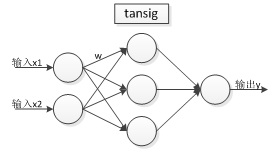
In this way, the structure is as shown in the following figure:

Among them,
the tansig function is a Sigmoid function: $\text{y} = \dfrac{2}{1+e^{-2x}} -1$

purelin is an identity linear mapping function: $\text{y}=x$

PASS:

1. The output layer is set to purelin, which means that the output layer has no activation function.
2. The hidden layer activation function can also be set to logsig: $\text{y} = \dfrac{1}{1+e^{-x}}$ , which is not much different from tansig. The difference is that the value range of logsig is [0, 1], while tansig is [-1, 1].

03. Mathematical structure of BP (expression)

Here, we do not provide general mathematical constructs,

Just use a simple example to describe its mathematical structure, which is more specific and easier to understand

There is an existing BP neural network, its structure is as follows:

An input layer, a hidden layer, and an output layer, and the number of nodes in the input layer, hidden layer, and output layer are [2, 3, 1] respectively.

Transfer function settings: hidden layer (tansig function). Output layer (purelin function).

The model topology is as follows:

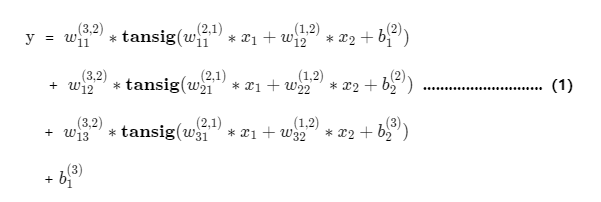
The mathematical expression can be written according to the model as follows:

PASS: There are many parameters in the expression, but there are actually only two types of parameters: weight w and threshold b.
$w_{12}^{(3,2)}$ It means that this weight is the weight from the second node of the second layer to the first node of the third layer.
$b_1^{(2)}$ Represents that this threshold is the threshold of the first node in layer 2.
Remarks: The subscript of the weight matrix w is generally from the back layer to the front layer, which is more concise when expressing the matrix

2. Gradient descent method to solve BP neural network

01. Problem

The following data are available:

y is actually generated $\color{blue}\text{y}=\text{sin}(x_1)+0.2*x_2^2$ by

Now, we need to train a neural network, fit it, and finally, we $\color{blue}\text{y}=\text{sin}(x_1)+0.2*x_2^2$ compare with

02. Modeling ideas

Set up the neural network structure

Here we set a hidden layer, 3 hidden neurons, and the activation function of the hidden layer is tansig,

then our network topology is as follows:

The corresponding mathematical expression of the model is:

Loss function and gradient

The loss function is:
$\displaystyle \textbf{E}(W,b)=\dfrac{1}{m}\sum \limits _{i=1}^{m} (\hat{\text{y}}_i-\text{y}_i)^2$

Hidden layer --> The weight of the output layer and the threshold gradient of the output layer are:

$\dfrac{\partial E}{\partial b^{(o)}} =\dfrac{\partial E}{\partial N^{(o)}}$

$\dfrac{\partial E}{\partial W^{(h-o)}} =\dfrac{\partial E}{\partial N^{(o)}} \left ( A^{(h)} \right )^T$

where, $A^{(h)}$ is the activation value of the hidden layer,

$\dfrac{\partial E}{\partial N^{(o)}}$ and is the node gradient of the output layer:

$\dfrac{\partial E}{\partial N^{(o)}} = \dfrac{2}{m*k} (\hat{\text{y}}-\text{y})$

Hidden layer --> The weight of the output layer and the threshold gradient of the hidden layer are:

$\dfrac{\partial E}{\partial b^{(h)}} =\dfrac{\partial E}{\partial N^{(h)}}$

$\dfrac{\partial E}{\partial W^{(i-h)}} =\dfrac{\partial E}{\partial N^{(h)}} \left ( A^{(i)} \right )^T =\dfrac{\partial E}{\partial N^{(h)}}X^{T}$

where, $\dfrac{\partial E}{\partial N^{(h)}}$ is the node gradient of the hidden layer:

$\dfrac{\partial E}{\partial N^{(h)}} = \left (W^{(h-o)}\right) ^T \dfrac{2}{m*k} (\hat{\text{y}}-\text{y}).*\left(1-\left ( A^{(h)} \right )^2 \right )$

Algorithm flow

Initialize W, b first,
(1) Calculate the gradient according to the gradient formula
(2) Adjust W to the negative gradient direction
Repeat (1) and (2) until the termination condition is reached (for example, the maximum number of iterations is reached, or the error is small enough)

03. Code implementation

close all;clear all;
%-----------数据----------------------
x1 = [-3,-2.7,-2.4,-2.1,-1.8,-1.5,-1.2,-0.9,-0.6,-0.3,0,0.3,0.6,0.9,1.2,1.5,1.8];% x1：x1 = -3:0.3:2;
x2 = [-2,-1.8,-1.6,-1.4,-1.2,-1,-0.8,-0.6,-0.4,-0.2,-2.2204,0.2,0.4,0.6,0.8,1,1.2]; % x2：x2 = -2:0.2:1.2;
X  = [x1;x2];      % 将x1,x2作为输入数据
y  = [0.6589,0.2206,-0.1635,-0.4712,-0.6858,-0.7975,-0.8040,...
    -0.7113,-0.5326,-0.2875 ,0.9860,0.3035,0.5966,0.8553,1.0600,1.1975,1.2618];    % y： y = sin(x1)+0.2*x2.*x2;

%--------参数设置与常量计算-------------
setdemorandstream(88);
hide_num = 3;
lr = 0.05;
[in_num,sample_num] = size(X);
[out_num,~] =  size(y);

%--------初始化w,b和预测结果-----------
w_ho = rand(out_num,hide_num);   % 隐层到输出层的权重 
b_o  = rand(out_num,1);          % 输出层阈值
w_ih = rand(hide_num,in_num);    % 输入层到隐层权重
b_h  = rand(hide_num,1);         % 隐层阈值
simy = w_ho*tansig(w_ih*X+repmat(b_h,1,size(X,2)))+repmat(b_o,1,size(X,2)); % 预测结果
mse_record = [sum(sum((simy - y ).^2))/(sample_num*out_num)];  % 预测误差记录

% ---------用梯度下降训练------------------
for i = 1:5000
    %计算梯度
    hide_Ac = tansig(w_ih*X+repmat(b_h,1,sample_num)); % 隐节点激活值
    dNo     = 2*(simy - y )/(sample_num*out_num);      % 输出层节点梯度
    dw_ho   = dNo*hide_Ac';                            % 隐层-输出层权重梯度
    db_o    = sum(dNo,2);                              % 输出层阈值梯度
    
    dNh     = (w_ho'*dNo).*(1-hide_Ac.^2);             % 隐层节点梯度
    dw_ih   = dNh*X';                                  % 输入层-隐层权重梯度
    db_h    = sum(dNh,2);                              % 隐层阈值梯度

    %往负梯度更新w,b
    w_ho = w_ho - lr*dw_ho;                            % 更新隐层-输出层权重 
    b_o  = b_o  - lr*db_o;                             % 更新输出层阈值
    w_ih = w_ih - lr*dw_ih;                            % 更新输入层-隐层权重 
    b_h  = b_h  - lr*db_h;                             % 更新隐层阈值
    
    % 计算网络预测结果与记录误差
    simy = w_ho*tansig(w_ih*X+repmat(b_h,1,size(X,2)))+repmat(b_o,1,size(X,2));
    mse_record =[mse_record, sum(sum((simy - y ).^2))/(sample_num*out_num)];
end

% -------------绘制训练结果与打印模型参数-----------------------------
h = figure;
subplot(1,2,1)
plot(mse_record)
subplot(1,2,2)
plot(1:sample_num,y);
hold on
plot(1:sample_num,simy,'-r');
set(h,'units','normalized','position',[0.1 0.1 0.8 0.5]);
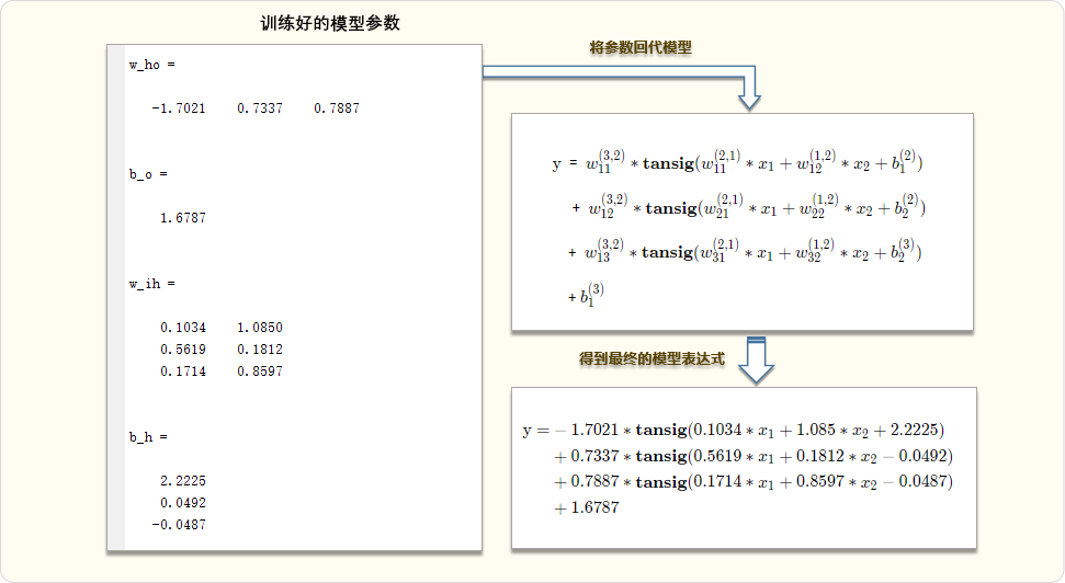
%--模型参数--
w_ho   % 隐层到输出层的权重 
b_o    % 输出层阈值
w_ih   % 输入层到隐层权重
b_h    % 隐层阈值

04. Running results

05. Check the effect of the model

Test with x = [0.5,0.5],

Model prediction results

$\begin{aligned} \text{y} =& -1.7021*\textbf{tansig}(0.1034*x_1+1.085*x_2+2.2225) \\ &+ 0.7337*\textbf{tansig}(0.5619*x_1+0.1812*x_2-0.0492) \\ &+ 0.7887*\textbf{tansig}(0.1714*x_1+0.8597*x_2-0.0487) \\&+1.6787\end{aligned}$

Substituting x =[0.5,0.5] into the above network model expression yields 0.6241

real result

Substituting x =[0.5,0.5] into the real relation $\text{y}=\sin(x_1)+0.2*x_{2}^{2}$ yields 0.5294.

Analysis of forecast results

The predicted value of the network is 0.6241 and the true value is 0.5294 with an error of 0.0946.
This error is not too large, but not too small.
Overall, the model training has a certain effect, indicating that the algorithm is feasible.
PASS: Why is the training data so good, but there is still such a big gap in the predicted value? Can readers figure it out? Can it be improved? How can it be improved?

Special statement: The realization of the entire solution process of the above gradient descent method is very rough, and it is only used as an introductory reference.

related articles

"BP Neural Network Gradient Derivation"

"Mathematical expressions extracted by BP neural network"

"A Complete Modeling Process of BP"

Gradient descent method to solve a simple demo of BP neural network

1. Introduction to BP model

01. BP structure and bionic ideas

02. Commonly used BP structure

03. Mathematical structure of BP (expression)

2. Gradient descent method to solve BP neural network

01. Problem

02. Modeling ideas

03. Code implementation

04. Running results

05. Check the effect of the model

Guess you like