Abstract: In order to evaluate the generalization ability of the model, that is, to judge whether the model is good or bad, we need to use a certain index to measure it. With the evaluation index, we can compare the pros and cons of different models, and use this index to further optimize the model. .
This article is shared from Huawei Cloud Community " Detailed Explanation of Evaluation Indicators and Code Implementation of Target Detection Model ", author: Embedded Vision.
foreword
In order to understand the generalization ability of the model, that is, to judge whether the model is good or bad, we need to use a certain index to measure it. With the evaluation index, we can compare the pros and cons of different models, and use this index to further optimize the model. For the two types of supervised models, classification and regression, there are separate evaluation criteria .
Different problems and different data sets will have different model evaluation indicators, such as classification problems. In the case of balanced data set categories, accuracy can be used as an evaluation indicator, but in reality, almost all data sets are unbalanced categories, so Generally, AP is used as the evaluation index of classification, the AP of each category is calculated separately, and then the mAP is calculated .
1. Precision, recall and F1
1.1, accuracy rate
Accuracy (precision) – Accuracy , the percentage of predicted correct results in the total samples, defined as follows:
Accuracy = ( TP + TN )/( TP + TN + FP + FN )
Error rate and precision, although commonly used, do not meet all task requirements. Take the watermelon problem as an example. Assuming that the melon farmer brings a cart of watermelons, we use the trained model to discriminate the watermelons. Now the accuracy can only measure how many watermelons are judged to be of the correct category (two categories: good melons and bad melons). ). But if we are more concerned about "what proportion of the picked watermelons are good melons", or "how many proportions of all good melons are picked", then the indicators of accuracy and error rate are obviously not enough.
Although the accuracy rate can judge the overall correct rate, it cannot be used as a good indicator to measure the result when the sample is unbalanced. To give a simple example, for example, in a total sample, positive samples account for 90%, negative samples account for 10%, and the samples are seriously unbalanced. In this case, we only need to predict all samples as positive samples to get a high accuracy rate of 90%, but in fact we didn't classify them very carefully, just casually. This shows that due to the problem of sample imbalance, the obtained high-accuracy results contain a lot of water. That is, if the samples are not balanced, the accuracy rate will be invalid.
1.2, precision rate, recall rate
The calculation of precision rate (precision rate) P and recall rate (recall rate) R involves the definition of confusion matrix. The confusion matrix table is as follows:
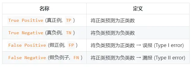
Precision and recall formulas:
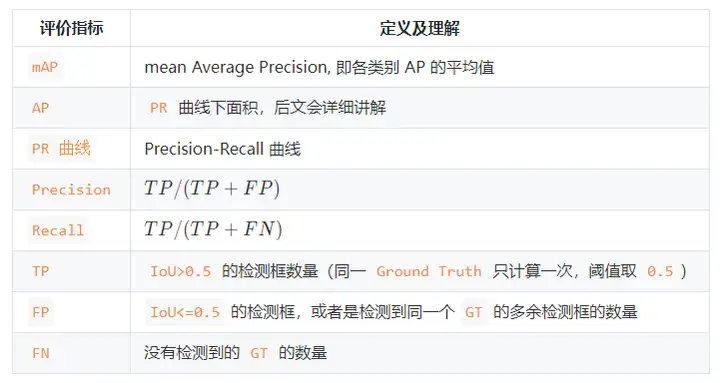
- Precision rate (precision rate) P=TP/(TP+FP) P = TP /( TP + FP )
- Recall rate (recall rate) R=TP/(TP+FN) R = TP /( TP + FN )
Precision rate and accuracy rate look somewhat similar, but they are two completely different concepts. The precision rate represents the prediction accuracy of the positive sample results, and the accuracy rate represents the overall prediction accuracy , including both positive samples and negative samples.
The precision rate describes how accurate the model is , that is, how many of the predicted positive examples are true examples; the recall rate describes how complete the model is , that is, how many of the true samples are predicted by our model is a positive example. The difference between the precision rate and the recall rate lies in the different denominators . One denominator is the number of samples predicted to be positive, and the other is the number of all positive samples in the original sample.
1.3, F1 score
If we want to find a balance between P and R , we need a new indicator: F 1 score. The F 1 score takes both the precision rate and the recall rate into account, so that the two can reach the highest at the same time, and a balance is taken. The calculation formula of F 1 is as follows:
The F 1 calculation here is for the binary classification model, please refer to the following for the calculation of F 1 for multi-classification tasks.

The general form of the F 1 metric: Fβ , which allows us to express our bias towards precision/recall, Fβ is calculated as follows:

Among them, β > 1 has a greater impact on the recall rate, and β < 1 has a greater impact on the precision rate.
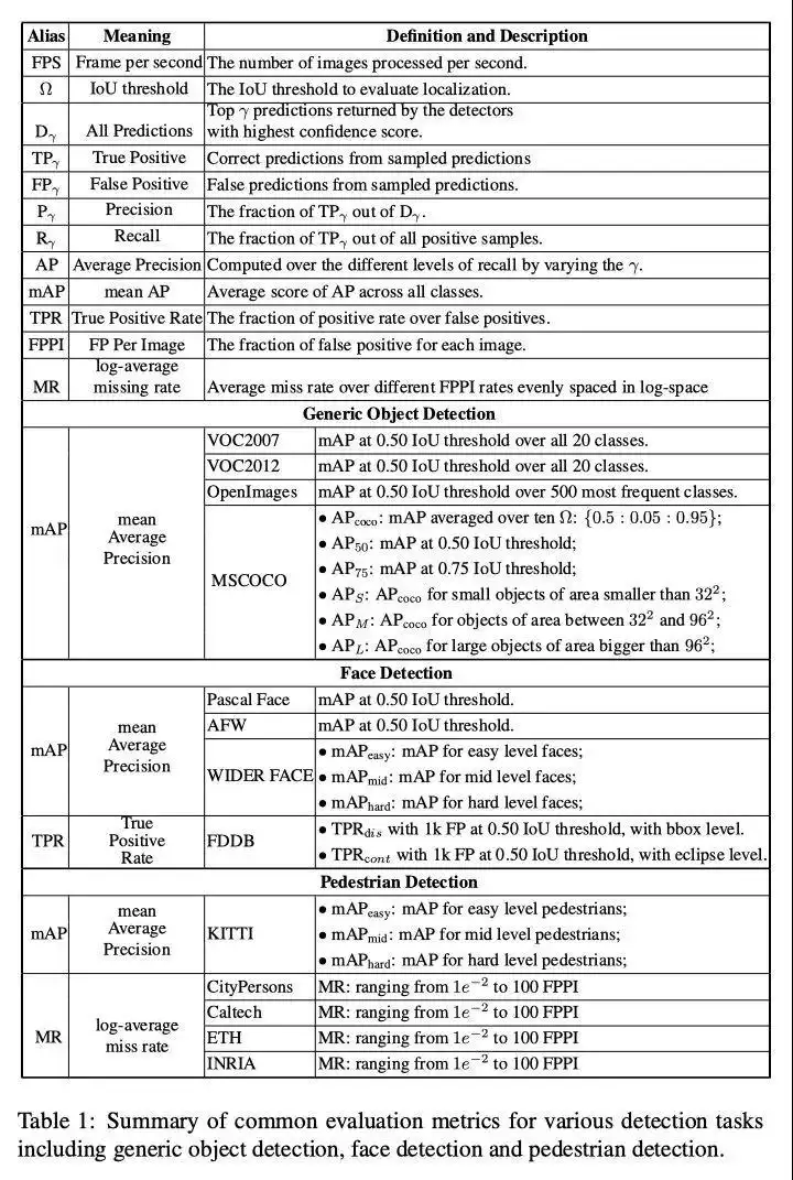
Different computer vision problems have different preferences for the two types of errors, and often try to reduce the other type of errors when a certain type of error is not more than a certain threshold. In target detection, mAP (mean Average Precision) takes both errors into consideration as a unified indicator.
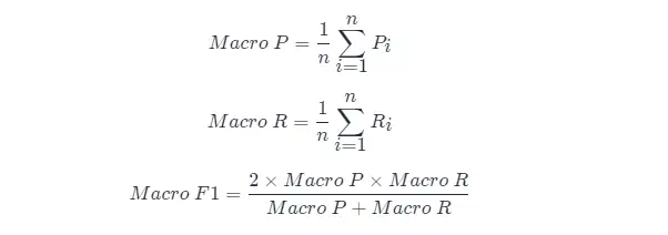
Many times we will have multiple confusion matrices, such as multiple training/testing, each time a confusion matrix can be obtained; or training/testing on multiple data sets, hoping to estimate the "global" performance of the algorithm; and Or to perform multi-classification tasks, each combination of two categories corresponds to a confusion matrix; ...In general, we hope to comprehensively consider the precision and recall rates on the n n two-category confusion matrices.
A direct approach is to first calculate the precision and recall rates on each confusion matrix, which are recorded as ( P 1, R 1), ( P 2, R 2),...,( Pn , Rn ) Then take the average, so that you get "Macro Precision (Macro-P)", "Macro Precision (Macro-R)" and the corresponding "Macro F1 F 1 (Macro- F1 ) ":
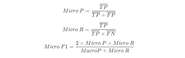
Another method is to average the corresponding elements of each confusion matrix to obtain the average values of TP, FP, TN, FN TP , FP , TN , and FN , and then calculate the "micro-precision rate" (Micro-P ), "Micro Recall" (Micro-R) and "Micro F 1" (Mairo-F1)
1.4, PR curve
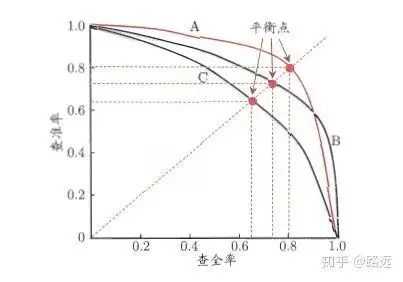
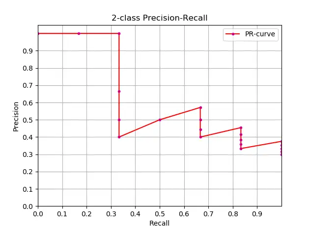
The relationship between the precision rate and the recall rate can be shown by a PR graph. Taking the precision rate P as the vertical axis and the recall rate R as the horizontal axis, you can get the precision rate-recall rate curve, referred to as the PR curve . The area under the PR curve is defined as AP:
1.4.1, How to understand the PR curve
It can be understood from a ranking model or a classification model. Taking logistic regression as an example, the output of logistic regression is a probability number between 0 and 1. Therefore, if we want to judge whether a user is good or bad according to this probability, we must define a threshold. Generally speaking, the greater the probability of logistic regression, the closer it is to 1, which means that he is more likely to be a bad user. For example, we define a threshold of 0.5, that is, we consider all users with a probability less than 0.5 to be good users, and those with a probability greater than 0.5 to be considered bad users. Therefore, for the threshold value of 0.5, we can get the corresponding pair of precision and recall.
But the problem is: this threshold is defined arbitrarily by us, and we don't know whether this threshold meets our requirements. Therefore, in order to find a most suitable threshold to meet our requirements, we must traverse all thresholds between 0 and 1, and each threshold corresponds to a pair of precision and recall, so we get PR curve.
Finally, how to find the best threshold point? First of all, we need to explain our requirements for these two indicators: we hope that both the precision rate and the recall rate are very high at the same time. But in fact, these two indicators are a pair of contradictions, and it is impossible to achieve double highs. It is obvious from the graph that if one of them is very high, the other must be very low. Selecting an appropriate threshold point depends on actual needs. For example, if we want a high recall rate, we will sacrifice some precision rate. In the case of ensuring the highest recall rate, the precision rate is not so low. .
1.5, ROC curve and AUC area
- The PR curve has Recall as the horizontal axis and Precision as the vertical axis; while the ROC curve has FPR as the horizontal axis and TPR as the vertical axis**. The closer the PR curve is to the upper right corner, the better the performance . Both metrics of the PR curve focus on positive examples
- The PR curve shows the Precision vs Recall curve, and the ROC curve shows the FPR (x-axis: False positive rate) vs TPR (True positive rate, TPR) curve.
- [ ] ROC curve
- [ ] AUC area
2. AP and mAP
2.1, Understanding of AP and mAP indicators
AP measures the quality of the trained model in each category, and mAP measures the quality of the model in all categories. After obtaining the AP, the calculation of mAP becomes very simple, which is to take the average of all APs . The calculation formula of AP is relatively complicated (so it is a separate chapter), please refer to the following for details.
The term mAP has different definitions. This metric is commonly used in the areas of information retrieval, image classification, and object detection. However, the two fields calculate mAP differently. Here we only talk about the mAP calculation method in object detection.
mAP is often used as an evaluation index for target detection algorithms. Specifically, for each picture detection model will output multiple prediction frames (far exceeding the number of real frames), we use IoU (Intersection Over Union) to Whether the prediction box of the mark prediction is accurate. After the marking is completed, the recall rate R will always increase with the increase of the prediction frame. The accuracy rate P is averaged at different recall rate R levels to obtain AP, and finally all categories are averaged according to their proportions. , that is, the mAP index is obtained.
2.2, Approximate calculation of AP
Knowing the definition of AP, the next step is to understand the realization of AP calculation. In theory, AP can be calculated by integral. The formula is as follows:

But usually, approximate or interpolation methods are used to calculate AP .
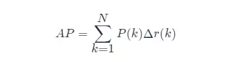
- Approximate calculation of AP (approximate average precision), this calculation method is approximated form;
- Obviously, points located on a vertical line do not contribute to the calculation of AP ;
- Here N is the total amount of data, k is the index of each sample point, Δ r ( k )= r ( k )− r ( k −1).
The code for approximate calculation of AP and drawing of PR curve is as follows:
import numpy as np
import matplotlib.pyplot as plt
class_names = ["car", "pedestrians", "bicycle"]
def draw_PR_curve(predict_scores, eval_labels, name, cls_idx=1):
 """calculate AP and draw PR curve, there are 3 types
    Parameters:
    @all_scores: single test dataset predict scores array, (-1, 3)
    @all_labels: single test dataset predict label array, (-1, 3)
    @cls_idx: the serial number of the AP to be calculated, example: 0,1,2,3...
    """
 # print('sklearn Macro-F1-Score:', f1_score(predict_scores, eval_labels, average='macro'))
 global class_names
    fig, ax = plt.subplots(nrows=1, ncols=1, figsize=(15, 10))
 # Rank the predicted scores from large to small, extract their corresponding index(index number), and generate an array
 idx = predict_scores[:, cls_idx].argsort()[::-1]
 eval_labels_descend = eval_labels[idx]
 pos_gt_num = np.sum(eval_labels == cls_idx) # number of all gt
 predict_results = np.ones_like(eval_labels)
 tp_arr = np.logical_and(predict_results == cls_idx, eval_labels_descend == cls_idx) # ndarray
 fp_arr = np.logical_and(predict_results == cls_idx, eval_labels_descend != cls_idx)
 tp_cum = np.cumsum(tp_arr).astype(float) # ndarray, Cumulative sum of array elements.
 fp_cum = np.cumsum(fp_arr).astype(float)
 precision_arr = tp_cum / (tp_cum + fp_cum) # ndarray
 recall_arr = tp_cum / pos_gt_num
    ap = 0.0
 prev_recall = 0
 for p, r in zip(precision_arr, recall_arr):
      ap += p * (r - prev_recall)
 # pdb.set_trace()
 prev_recall = r
 print("------%s, ap: %f-----" % (name, ap))
 fig_label = '[%s, %s] ap=%f' % (name, class_names[cls_idx], ap)
 ax.plot(recall_arr, precision_arr, label=fig_label)
 ax.legend(loc="lower left")
 ax.set_title("PR curve about class: %s" % (class_names[cls_idx]))
 ax.set(xticks=np.arange(0., 1, 0.05), yticks=np.arange(0., 1, 0.05))
 ax.set(xlabel="recall", ylabel="precision", xlim=[0, 1], ylim=[0, 1])
 fig.savefig("./pr-curve-%s.png" % class_names[cls_idx])
 plt.close(fig)
2.3, interpolation calculation AP
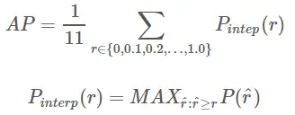
The evolution process of the formula of Interpolated average precision AP AP will not be discussed here. For details, please refer to this article. The formulas and diagrams here are also referred to this article. 11-point interpolation calculation method to calculate AP AP formula is as follows:
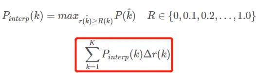
- This is the AP in the usual sense of 11 points_Interpolated form, select fixed 0,0.1,0.2,…,1.00,0.1,0.2,…,1.0 11 thresholds, this is used in PASCAL2007
- Here, because there are only 11 points involved in the calculation, K = 11, called 11 points_Interpolated, and k is the threshold index
- Pinterp ( k ) takes the maximum value in the sample after the sample point corresponding to the kth threshold, except that the threshold here is limited to the range of 0,0.1,0.2,…,1.00,0.1,0.2,…, 1.0 Inside.
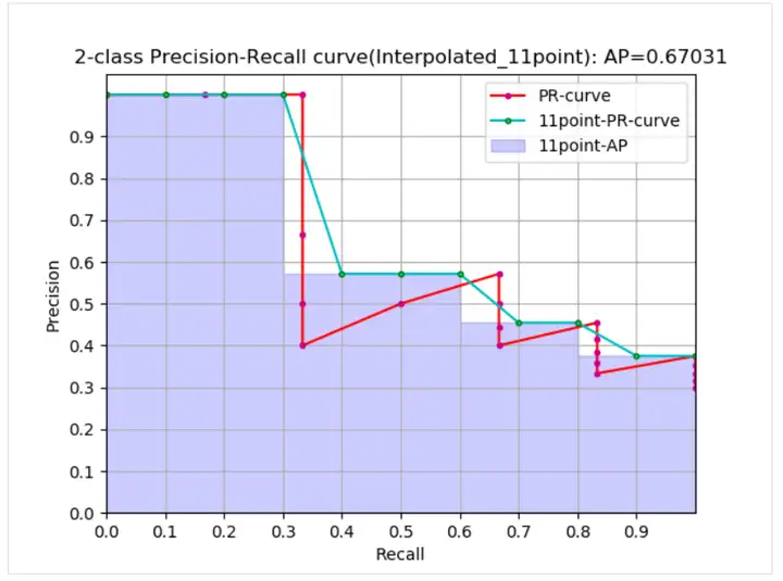
From the curve, the real AP< approximated AP < Interpolated AP, 11-points Interpolated AP may be large or small, and when the amount of data is large, it will be close to Interpolated AP. Unlike Interpolated AP, AP is calculated in the previous formula. It is the area estimate of the PR curve. The formula given in the PASCAL paper is simpler and more crude, directly calculating the average value of the precision at 11 thresholds. The 11-point formula for calculating AP given in the PASCAL paper is as follows.
1. Calculate AP under the given conditions of recal and precision:
def voc_ap(rec, prec, use_07_metric=False):
 """
    ap = voc_ap(rec, prec, [use_07_metric])
    Compute VOC AP given precision and recall.
    If use_07_metric is true, uses the
    VOC 07 11 point method (default:False).
    """
 if use_07_metric:
 # 11 point metric
        ap = 0.
 for t in np.arange(0., 1.1, 0.1):
 if np.sum(rec >= t) == 0:
                p = 0
 else:
                p = np.max(prec[rec >= t])
            ap = ap + p / 11.
 else:
 # correct AP calculation
 # first append sentinel values at the end
 mrec = np.concatenate(([0.], rec, [1.]))
 mpre = np.concatenate(([0.], prec, [0.]))
 # compute the precision envelope
 for i in range(mpre.size - 1, 0, -1):
 mpre[i - 1] = np.maximum(mpre[i - 1], mpre[i])
 # to calculate area under PR curve, look for points
 # where X axis (recall) changes value
 i = np.where(mrec[1:] != mrec[:-1])[0]
 # and sum (\Delta recall) * prec
        ap = np.sum((mrec[i + 1] - mrec[i]) * mpre[i + 1])
 return ap
2. Calculate AP given target detection result file and test set label file xml:
def parse_rec(filename):
 """ Parse a PASCAL VOC xml file
 Return : list, element is dict.
    """
    tree = ET.parse(filename)
    objects = []
 for obj in tree.findall('object'):
 obj_struct = {}
 obj_struct['name'] = obj.find('name').text
 obj_struct['pose'] = obj.find('pose').text
 obj_struct['truncated'] = int(obj.find('truncated').text)
 obj_struct['difficult'] = int(obj.find('difficult').text)
 bbox = obj.find('bndbox')
 obj_struct['bbox'] = [int(bbox.find('xmin').text),
 int(bbox.find('ymin').text),
 int(bbox.find('xmax').text),
 int(bbox.find('ymax').text)]
 objects.append(obj_struct)
 return objects
def voc_eval(detpath,
 annopath,
 imagesetfile,
 classname,
 cachedir,
 ovthresh=0.5,
             use_07_metric=False):
 """rec, prec, ap = voc_eval(detpath,
 annopath,
 imagesetfile,
 classname,
                                [ovthresh],
                                [use_07_metric])
    Top level function that does the PASCAL VOC evaluation.
 detpath: Path to detections result file
 detpath.format(classname) should produce the detection results file.
 annopath: Path to annotations file
 annopath.format(imagename) should be the xml annotations file.
 imagesetfile: Text file containing the list of images, one image per line.
 classname: Category name (duh)
 cachedir: Directory for caching the annotations
    [ovthresh]: Overlap threshold (default = 0.5)
    [use_07_metric]: Whether to use VOC07's 11 point AP computation
        (default False)
    """
 # assumes detections are in detpath.format(classname)
 # assumes annotations are in annopath.format(imagename)
 # assumes imagesetfile is a text file with each line an image name
 # cachedir caches the annotations in a pickle file
 # first load gt
 if not os.path.isdir(cachedir):
 os.mkdir(cachedir)
 cachefile = os.path.join(cachedir, '%s_annots.pkl' % imagesetfile)
 # read list of images
 with open(imagesetfile, 'r') as f:
        lines = f.readlines()
 imagenames = [x.strip() for x in lines]
 if not os.path.isfile(cachefile):
 # load annotations
        recs = {}
 for i, imagename in enumerate(imagenames):
            recs[imagename] = parse_rec(annopath.format(imagename))
 if i % 100 == 0:
 print('Reading annotation for {:d}/{:d}'.format(
 i + 1, len(imagenames)))
 # save
 print('Saving cached annotations to {:s}'.format(cachefile))
 with open(cachefile, 'wb') as f:
 pickle.dump(recs, f)
 else:
 # load
 with open(cachefile, 'rb') as f:
 try:
                recs = pickle.load(f)
 except:
                recs = pickle.load(f, encoding='bytes')
 # extract gt objects for this class
 class_recs = {}
 npos = 0
 for imagename in imagenames:
        R = [obj for obj in recs[imagename] if obj['name'] == classname]
 bbox = np.array([x['bbox'] for x in R])
        difficult = np.array([x['difficult'] for x in R]).astype(np.bool)
        det = [False] * len(R)
 npos = npos + sum(~difficult)
 class_recs[imagename] = {'bbox': bbox,
 'difficult': difficult,
 'det': det}
 # read dets
 detfile = detpath.format(classname)
 with open(detfile, 'r') as f:
        lines = f.readlines()
 splitlines = [x.strip().split(' ') for x in lines]
 image_ids = [x[0] for x in splitlines]
    confidence = np.array([float(x[1]) for x in splitlines])
    BB = np.array([[float(z) for z in x[2:]] for x in splitlines])
 nd = len(image_ids)
 tp = np.zeros(nd)
 fp = np.zeros(nd)
 if BB.shape[0] > 0:
 # sort by confidence
 sorted_ind = np.argsort(-confidence)
 sorted_scores = np.sort(-confidence)
        BB = BB[sorted_ind, :]
 image_ids = [image_ids[x] for x in sorted_ind]
 # go down dets and mark TPs and FPs
 for d in range(nd):
            R = class_recs[image_ids[d]]
            bb = BB[d, :].astype(float)
 ovmax = -np.inf
            BBGT = R['bbox'].astype(float)
 if BBGT.size > 0:
 # compute overlaps
 # intersection
 ixmin = np.maximum(BBGT[:, 0], bb[0])
 iymin = np.maximum(BBGT[:, 1], bb[1])
 ixmax = np.minimum(BBGT[:, 2], bb[2])
 iymax = np.minimum(BBGT[:, 3], bb[3])
 iw = np.maximum(ixmax - ixmin + 1., 0.)
 ih = np.maximum(iymax - iymin + 1., 0.)
                inters = iw * ih
 # union
 uni = ((bb[2] - bb[0] + 1.) * (bb[3] - bb[1] + 1.) +
 (BBGT[:, 2] - BBGT[:, 0] + 1.) *
 (BBGT[:, 3] - BBGT[:, 1] + 1.) - inters)
                overlaps = inters / uni
 ovmax = np.max(overlaps)
 jmax = np.argmax(overlaps)
 if ovmax > ovthresh:
 if not R['difficult'][jmax]:
 if not R['det'][jmax]:
 tp[d] = 1.
                        R['det'][jmax] = 1
 else:
 fp[d] = 1.
 else:
 fp[d] = 1.
 # compute precision recall
 fp = np.cumsum(fp)
 tp = np.cumsum(tp)
    rec = tp / float(npos)
 # avoid divide by zero in case the first detection matches a difficult
 # ground truth
 prec = tp / np.maximum(tp + fp, np.finfo(np.float64).eps)
    ap = voc_ap(rec, prec, use_07_metric)
 return rec, prec, ap
2.4, mAP calculation method
Because the calculation of the mAP value is to average the AP values of all categories in the data set , so we want to calculate the mAP , we must first know how to find the AP value of a certain category . The AP calculation methods of a certain category of different data sets are similar, mainly divided into three types:
(1) In VOC2007, you only need to select the maximum value of Precision when Recall>=0,0.1,0.2,...,1 Recall >=0,0.1,0.2,...,1, a total of 11 points, and then AP AP is the average of these 11 Precisions, and mAP mAP is the average of all AP AP values of all categories. The code for calculating AP AP in the VOC dataset (using the interpolation calculation method, the code comes from the py-faster-rcnn warehouse )
(2) In VOC2010 and later, for each different Recall value (including 0 and 1), it is necessary to select the maximum value of Precision when it is greater than or equal to these Recall values, and then calculate the area under the PR curve as the AP value, mAP mAP is all The average of category AP values.
(3) For the COCO data set, set multiple IOU thresholds (0.5-0.95, 0.05 is the step size), and there is a certain category of AP value under each IOU threshold, and then calculate the AP average under different IOU thresholds, that is The desired final AP value of a category.
3. Summary of Target Detection Metrics
Fourth, reference materials
- Target detection evaluation standard-AP mAP
- Performance Evaluation Metrics for Object Detection
- Soft-NMS
- Recent Advances in Deep Learning for Object Detection
- A Simple and Fast Implementation of Faster R-CNN
- Classification model evaluation indicators - accuracy rate, precision rate, recall rate, F1, ROC curve, AUC curve
- This article gives you a thorough understanding of accuracy, precision, recall, true rate, false positive rate, ROC/AUC
Click to follow and learn about Huawei Cloud's fresh technologies for the first time~