Translation: Transfer learning Transfer Learning Guide

Here's everything you need to know about classic transfer learning and deep transfer learning. Read this guide to improve your model training and get better performance in less time.

1. Background

Here's the thing -

Collecting large amounts of data when tackling a brand new task can be challenging, to say the least.

However-

Getting satisfactory model performance (think: model accuracy) using only a limited amount of training data is also tricky...if not impossible.

Fortunately, there is a solution to this problem, and it's called transfer learning.

This is almost too good to be true because the idea is very simple: you can train a model with a small amount of data and still achieve a high level of performance.

Cool, right? Well, read on as we'll give you the best explanation of how it all works.

2. What is transfer learning?

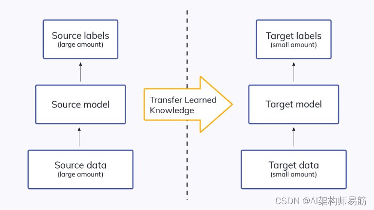
Transfer learning is a machine learning method where we reuse pre-trained models as a starting point for models for new tasks.

In short, a model trained on one task is reused for a second related task, as an optimization, allowing rapid progress in modeling the second task.

By applying transfer learning to a new task, significantly higher performance can be achieved compared to training with only a small amount of data.

Transfer learning is so common that models are rarely trained from scratch for tasks related to image or natural language processing.

Instead, researchers and data scientists prefer to start with a pre-trained model that already knows how to classify objects and that has learned general features like edges, shapes, etc. in images.

ImageNet, AlexNet, and Inception are typical examples of models with a transfer learning foundation.

3. Traditional machine learning and transfer learning

Deep learning experts introduced transfer learning to overcome the limitations of traditional machine learning models.

Let's take a look at the difference between these two learning styles.

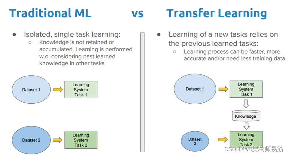
1. Traditional machine learning models need to be trained from scratch, are computationally intensive, and require large amounts of data to achieve high performance. On the other hand, transfer learning is computationally efficient and helps to achieve better results with small datasets.

2. Traditional machine learning has an isolated training approach, where each model is independently trained for a specific purpose without relying on past knowledge. In contrast, transfer learning uses knowledge gained from pretrained models to complete tasks. To better describe it:

You cannot use ImageNet's pretrained models with biomedical images because ImageNet does not contain images that belong to the biomedical domain.

3. Transfer learning models reach optimal performance faster than traditional machine learning models. This is because the features are already understood by the model using knowledge (features, weights, etc.) from previously trained models. It is faster than training a neural network from scratch.
   

4. Classical Transfer Learning Strategies

Apply different transfer learning strategies and techniques depending on the domain of the application, the task at hand, and the availability of data.

Before deciding on a transfer learning strategy, it is critical to answer the following questions:

• Which part of the knowledge can be transferred from the source to the target to improve the performance of the target task?
• When to migrate and when not to migrate in order to improve the performance/results of the target tasks without degrading them?
• How to transfer the knowledge gained from the source model according to our current domain/task?

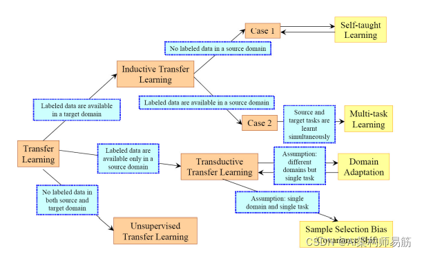
Traditionally, transfer learning strategies fall into three broad categories based on the task domain and the amount of labeled/unlabeled data present.
Let's explore them in more detail.

4.1 Inductive Transfer Learning

Inductive transfer learning requires the source and target domains to be the same, although the specific tasks handled by the models are different.

The algorithm tries to use the knowledge from the source model and apply it to improve the target task. A pretrained model already has expertise in domain features and is in a better starting point than if we were to train it from scratch.

Inductive transfer learning is further divided into two subcategories based on whether the source domain contains labeled data. These include multi-task learning and self-paced learning, respectively.

4.2 Transductive Transfer Learning

Scenarios where the domains of the source and target tasks are not identical but interrelated use a transductive transfer learning strategy. The similarity between the source task and the target task can be derived. These scenarios usually have a lot of labeled data in the source domain and only unlabeled data in the target domain.

4.3 Unsupervised Transfer Learning

Unsupervised transfer learning is similar to inductive transfer learning. The only difference is that the algorithm focuses on unsupervised tasks and involves unlabeled datasets in both source and target tasks.

5. Common methods of transfer learning

We will now take another approach to classify transfer learning strategies based on domain similarity, independent of the type of data samples used for training.

5.1 Homogeneous Transfer Learning

Homogeneous transfer learning methods are developed and proposed to handle the case where domains share the same feature space.

In isomorphic transfer learning, the marginal distributions of domains differ only slightly. These methods adjust the domain by correcting for sample selection bias or covariate shift.

This is a malfunction.

5.2 Instance transfer

It covers a simple scenario where there is a large amount of labeled data in the source domain and a limited amount of labeled data in the target domain. Both domain and feature space differ only in marginal distributions.

For example, let's say we need to build a model to diagnose cancer in a specific area where the elderly are the majority. A limited number of target domain instances are given, and relevant data are available from another region with a majority of young people. Transferring all data directly from another region may not be successful due to marginal distribution differences, and older adults have a higher risk of cancer than younger adults.

In this case, it is natural to consider adjusting the marginal distribution. Instance-based transfer learning reassigns weights to source domain instances in the loss function.

5.3 Parameter transfer

Parameter-based transfer learning methods transfer knowledge at the model/parameter level.

This approach involves transferring knowledge through shared parameters of source and target domain learner models. One way to transfer learned knowledge is to create multiple source learner models and optimally combine reweighted learners similar to ensemble learners to form an improved target learner.

The idea behind parameter-based methods is that a model well trained on the source domain has learned a well-defined structure that can be transferred to the target model if the two tasks are related. Generally speaking, there are two ways of weight sharing in deep learning models: soft weight sharing and hard weight sharing.

• In soft weight sharing, the model is expected to approximate the learned features and is usually penalized if its weights deviate significantly from a given set of weights.
• In hard weight sharing, we share the exact weights between different models.

5.4 Feature-representation transfer

Feature-based methods transform original features to create new feature representations. This approach can be further divided into two subcategories, namely asymmetric and symmetric feature-based transfer learning.

• Asymmetric methods transform source features to match target features. In other words, we take features from the source domain and fit them into the target feature space. Due to marginal differences in feature distributions, some information may be lost in the process.
• Symmetric methods find a common latent feature space and then transform both source and target features into this new feature representation.

5.5 Relational-knowledge transfer

Relation-based transfer learning methods mainly focus on learning the relationship between the source and target domains, and use this knowledge to derive past knowledge and use it in the current context.

This approach transfers logical relationships or rules learned in the source domain to the target domain.

For example, if we understand the relationship between different elements of speech in a male voice, it helps to analyze sentences in another voice.

5.6 Heterogeneous Transfer Learning

Transfer learning involves deriving representations from previous networks to extract meaningful features from new samples to accomplish interrelated tasks. However, these methods forget to consider the difference in feature space between the source and target domains.

Collecting labeled source domain data with the same feature space as the target domain is often challenging, and heterogeneous transfer learning methods have been developed to address these limitations.

This technique aims to solve the problem that the source and target domains have different feature spaces and other issues such as different data distributions and label spaces. Heterogeneous transfer learning is applied to cross-domain tasks such as cross-language text classification, text-to-image classification, etc.

6. Transfer Learning for Deep Learning

Finally, let's discuss transfer learning in the context of deep learning.

Fields such as natural language processing and image recognition are considered hot research areas for transfer learning. There are also many models that achieve state-of-the-art performance.

These pretrained neural networks/models form the basis of transfer learning in the context of deep learning, known as deep transfer learning.

6.1 Off-the-shelf pre-trained models as feature extractors

To understand the flow of deep learning models, it is necessary to understand their components.

Deep learning systems are layered architectures that can learn different features at different layers. The initial layers compile higher-level features, which shrink to fine-grained features as we go deeper into the network.

These layers are finally connected to the last layer (usually a fully connected layer, in the case of supervised learning) to obtain the final output. This opens the scope of using popular pretrained networks (e.g. Oxford VGG model, Google Inception model, Microsoft ResNet model) without having its last layer as a fixed feature extractor for other tasks.

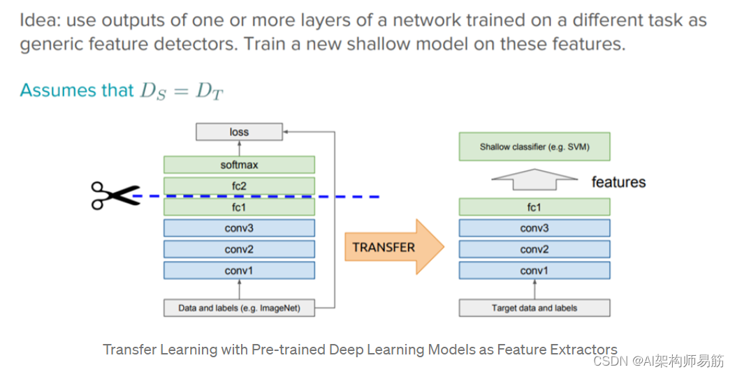
The key idea here is to utilize the weighted layers of the pretrained model to extract features instead of updating the model's weights with new data during training for new tasks.

A pretrained model is trained on a dataset large enough and general enough and will effectively serve as a general model for the visual world.

6.2 Fine Tuning Off-the-shelf Pre-trained Models

This is a more attractive technique, where we not only directly rely on the features extracted from the pretrained model and replace the last layer, but also selectively retrain some of the previous layers.

Deep neural networks are hierarchical structures with many tunable hyperparameters. The role of the initial layers is to capture generic features, while the later layers focus more on the explicit task at hand. It makes sense to fine-tune higher-order feature representations in the base model to make them more relevant to specific tasks. We can retrain certain layers of the model while maintaining some freeze during training.

The figure below depicts an example on an object detection task, where the initial lower layers of the network learn very general features, while the higher layers learn very task-specific features.

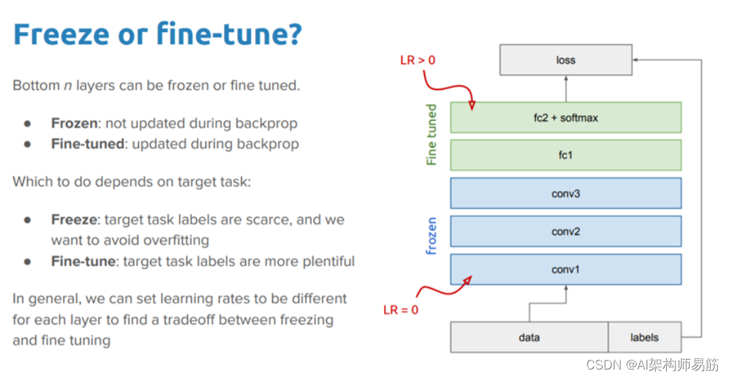
6.3 Freezing vs. Fine-tuning

A logical way to further improve the performance of your model is to retrain (or "fine-tune") the weights on the top layers of the pretrained model at the same time as training the classifier you added.

This forces the weights to be updated from the generic feature map that the model learns from the source task. Fine-tuning will allow the model to apply past knowledge in the target domain and relearn something again.

Also, one should try to fine-tune a few top layers rather than the entire model. The first few layers learn basic and generic features that generalize to almost all types of data.

Therefore, it is wise to freeze these layers and reuse basic knowledge gained from past training. As we get higher, these features become more and more specific to the dataset on which the model was trained. Fine-tuning aims to tune these special features to work with new datasets, not to cover general learning.

7. Transfer learning in 6 steps

Finally, let us walk you through how transfer learning works in practice.

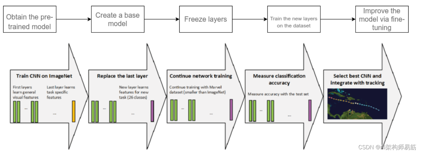
7.1. Obtain pre-trained model

The first step is to choose the pretrained model we wish to keep as a basis for training based on the task. Transfer learning requires a strong correlation between the knowledge of the pre-trained source model and the target task domain to make them compatible.

Here are some pretrained models you can use:

For computer vision :

• VGG-16
• VGG-19
• Inception V3
• XCeption
• ResNet-50

For NLP tasks :

• Word2Vec
• GloVe
• FastText

7.2. Create a base model

The base model is one of the architectures we chose in the first step that is closely related to our task, such as ResNet or Xception. We can download the network weights, which saves time for additional training of the model. Otherwise, we would have to train our model from scratch using the network architecture.

In some cases, the base model may have more neurons in the final output layer than we need in our use case. In this case, we need to remove the final output layer and make the corresponding changes.

7.3. Freeze layers

Freezing the starting layers from the pretrained model is crucial to avoid extra work for the model to learn basic features.

If we don't freeze the initial layer, we will lose all learning that has happened. This is no different than training a model from scratch and wastes time, resources, etc.

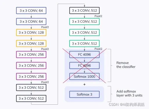
7.4. Add new trainable layers

The only knowledge we reuse from the base model is the feature extraction layer. We need to add extra layers on top of them to predict the special task of the model. These are usually the final output layers.

7.5. Train the new layers

The final output of the pretrained model is likely to be different from the model output we want. For example, a pretrained model trained on the ImageNet dataset will output 1000 classes.

However, we need our model to work for both classes. In this case, we have to train the model with a new output layer.

7.6. Fine-tune your model

One way to improve performance is fine-tuning.

Fine-tuning consists of unfreezing parts of the base model and retraining the entire model on the entire dataset with a very low learning rate. A low learning rate will improve the performance of the model on new datasets while preventing overfitting.

8. Types of Deep Transfer Learning

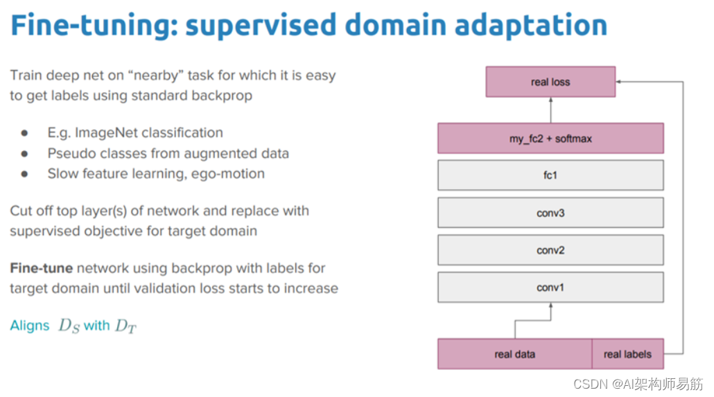
8.1 Domain Adaptation

Domain adaptation is a transfer learning scenario where the source and target domains have different feature spaces and distributions.

Domain adaptation is the process of adapting one or more source domains to convey information to improve the performance of the target learner. This process attempts to change the source domain to bring the source's distribution closer to the target's distribution.

8.2 Domain Confusion

In a neural network, different layers identify features of different complexity. In a perfect scenario, we would develop an algorithm that keeps this feature domain unchanged and improves its transferability across domains.

In such a context, the feature representations between the source and target domains should be as similar as possible. The goal is to add a target to the model at the source to encourage similarity to the target by obfuscating the source domain itself.

Specifically, the domain confusion loss is used to confuse the high-level classification layers of the neural network by matching the distributions of the target and source domains.

Finally, we want to make sure that the samples are indistinguishable to the classifier. To do this, the classification loss for source samples must be minimized, and the domain confusion loss for all samples must also be minimized.

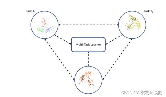
8.3 Multi-task Learning

In the case of multi-task learning, multiple tasks from the same domain are learned simultaneously without distinguishing between source and target.

We have a set of learning tasks t1 , t2 , ..., t(n)and we learn all tasks together at the same time.

This helps to transfer knowledge from each scenario and develop rich combined feature vectors from all different scenarios in the same domain. The learner optimizes the learning/performance of all n tasks with some shared knowledge.

8.4 One-shot Learning

One-shot learning is a classification task where we have one or a few examples to learn and classify many new examples in the future.

This is the case with face recognition, where faces must be correctly classified with different facial expressions, lighting conditions, accessories, and hairstyles, and the model has one or several template photos as input.

For one-shot learning, we need to rely entirely on knowledge transfer from base models trained on some examples we provide to a class.

8.5 Zero-shot Learning

If transfer learning overuses zero instances of a class and does not rely on labeled data samples, the corresponding strategy is called zero-shot learning.

Zero-shot learning requires additional data during the training phase to understand unseen data.

Zero-shot learning focuses on traditional input variables x, traditional output variables y, and task-specific random variables. Zero-shot learning comes in handy in scenarios like machine translation, where we may not have labels in the target language.

9. Deep Transfer Learning Applications

Transfer learning helps data scientists learn from knowledge gained from previously used machine learning models to accomplish similar tasks.

That's why this technology is now used in several areas that we list below.

9.1 Natural Language Processing NLP

NLP is one of the most attractive applications of transfer learning. Transfer learning uses knowledge from pretrained AI models that can understand language structure to solve cross-domain tasks. Daily NLP tasks such as next word prediction, question answering, and machine translation use deep learning models such as BERT, XLNet, Albert, and TF general models.

9.2 Computer Vision

Transfer learning is also applied to image processing.

Deep neural networks are used to solve image-related tasks because they are good at identifying complex features of images. The dense layers contain the logic to detect the image; therefore, adjusting the higher layers does not affect the underlying logic. Image recognition, object detection, image noise removal, etc. are typical application areas of transfer learning, as all image-related tasks require familiarity with basic knowledge of images and pattern detection.

9.3 Audio/Voice Audio/Speech

Transfer learning algorithms are used to solve audio/speech related tasks such as speech recognition or speech-to-text translation.

When we say "Siri" or "Hey Google!", the main AI model developed for English speech recognition is busy processing our commands on the backend.

Interestingly, the pretrained AI model developed for English speech recognition forms the basis of the French speech recognition model.

10. Transfer learning in short: key takeaways

Finally, let's do a quick recap of everything we've learned today. Here's a high-level summary of what we covered:

• Transfer learning models focus on storing knowledge gained while solving one problem and applying it to different but related problems.
• Instead of training a neural network from scratch, many pretrained models can be used as a starting point for training. These pre-trained models provide more reliable architectures and save time and resources.
• Transfer learning is used in scenarios where there is not enough data for training or we want to get better results in a short time.
• Transfer learning involves selecting a source model that is similar to the target domain, adapting the source model to the target model before knowledge transfer, and training the source model to achieve the target model.
• The higher layers of the model are usually fine-tuned, while the lower layers are frozen because the fundamentals of transferring from a source task to a target task in the same domain are the same.
• In tasks with a small amount of data, if the source model is too similar to the target model, there may be an overfitting problem. To prevent the transfer learning model from overfitting, having to adjust the learning rate, freezing some layers in the source model, or adding a linear classifier while training the target model can help avoid this problem.

reference

https://www.v7labs.com/blog/transfer-learning-guide