Recently, I was studying data structures and algorithms, and found Xiao Turtle's "Data Structure and Algorithms Course" in Station B, which is very interesting!
(Little Turtle) Data Structures and Algorithms
For an algorithm, the analysis has two steps, the first step is to prove the correctness of the algorithm mathematically, and the second step is to analyze the time complexity of the algorithm.
The time complexity of an algorithm reflects the magnitude of the increase in program execution time with the growth of the input scale, and to a large extent reflects the merits of the algorithm.
There are generally two ways to measure the execution time of a program.
The method of ex post statistics
This method has two flaws:
1. In order to evaluate the running performance of the designed algorithm, the corresponding program must first be compiled and run according to the algorithm;
2. The obtained statistics depend on environmental factors such as computer hardware and software, and sometimes it is easy to conceal the advantages of the algorithm itself.
Second, the method of pre-analysis and estimation
The time a program written in a high-level language takes to run on a computer depends on the following factors:
- The strategy and method adopted by the algorithm;
- The quality of the compiled code;
- the input size of the problem;
- The speed specified by the machine execution line;
An algorithm is composed of control structures (sequences, branches, and loops) and primitive operations (referring to operations of inherent data types), and the algorithm time depends on the combined effect of the two. In order to facilitate the comparison of different algorithms for the same problem, the usual practice is to select an original operation from the algorithm that is the basic operation for the problem (or type of algorithm) under study, and use the number of repeated executions of the basic operation as the The time measure of the algorithm.
3. Time complexity
1. Time frequency
The time consumed by the execution of an algorithm cannot be calculated theoretically, and it must be run on the computer to know it. But it is impossible and unnecessary for us to test every algorithm on the computer . We just need to know which algorithm takes more time and which algorithm takes less time. And the time spent by an algorithm is proportional to the number of executions of the statements in the algorithm, whichever algorithm has more statements executed, it takes more time. The number of executions in a statement in an algorithm is called the statement frequency or time frequency, denoted as T(n).
2. Time complexity
n is called the size of the problem, and when n keeps changing, the time frequency T(n) also keeps changing.
In general, the number of repetitions of the basic operations in the algorithm is a function of the problem size n, which is represented by T(n). If there is an auxiliary function f(n), when n approaches infinity, T(n The limit value of )/f(n) is a constant not equal to zero, then f(n) is said to be a function of the same order of magnitude as T(n). Denoted as T(n)=O(f(n)), O(f(n)) is called the asymptotic time complexity of the algorithm, referred to as the time complexity.
The role of the Landau notation is to describe the behavior of complex functions with simple functions, giving an upper and lower bound.
T (n) = Ο(f (n)) means that there is a constant C such that as n approaches positive infinity there is always T (n) ≤ C * f(n). Simply put, T(n) is as large as f(n) when n tends to positive infinity. That is, the upper bound on T(n) is C * f(n) as n approaches positive infinity. Although there is no requirement for f(n), it generally takes the simplest function possible. For example, O(2n2+n+1) = O (3n2+n+3) = O (7n2 + n) = O ( n2 ), generally only O(n2) is enough. Note that there is a constant C hidden in the big O notation, so no coefficients are generally added to f(n). If T(n) is regarded as a tree, then what O(f(n)) expresses is the trunk, only the trunk is concerned, and all other details are discarded.
Common time complexities are:
Constant order O(1) , logarithmic order O( log 2n ), linear order O(n), linear logarithmic order O( n log 2n ), square order O( n 2), cubic order O( n 3 ) ,..., k-th power order O( n k), exponential order O( 2 n). With the continuous increase of the problem size n, the above-mentioned time complexity continues to increase, and the execution efficiency of the algorithm is lower.
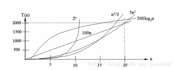
The time complexity of common algorithms from small to large is: Ο(1)<Ο(log 2n )<Ο(n)<Ο(nlog 2n )<Ο( n 2)<Ο( n 3)<…<Ο ( 2 n)<Ο(n!)
In general, for a problem (or a class of algorithms), only one basic operation needs to be selected to discuss the time complexity of the algorithm. Sometimes, several basic operations need to be considered at the same time, and different operations can even be given different weights. value to reflect the relative time required to perform different operations, which facilitates a comprehensive comparison of two completely different algorithms that solve the same problem.
3. The specific steps to solve the time complexity of the algorithm:
(1) Find the basic statement in the algorithm
The statement that executes the most times in the algorithm is the basic statement, usually the body of the innermost loop.
(2) Calculate the order of magnitude of the number of executions of the basic statement
It is only necessary to calculate the order of magnitude of the number of executions of the basic statement, which means that as long as the highest power in the function of the number of basic statement executions is guaranteed to be correct, all coefficients of the lower and highest powers can be ignored. This simplifies algorithm analysis and focuses attention on what matters most: growth rates.
(3) Use Big O notation to represent the time performance of the algorithm
Put the order of magnitude of the number of times the base statement is executed into big-O notation
If the algorithm contains nested loops, the base statement is usually the innermost loop body, and if the algorithm contains parallel loops, add the time complexity of the parallel loops.
Ο(1) indicates that the number of executions of the basic statement is a constant. Generally speaking, as long as there is no loop statement in the algorithm, the time complexity is Ο(1). where Ο( log 2n ), Ο(n), Ο( n log 2 n ), Ο( n 2) and Ο( n 3) are called polynomial time, and Ο( 2 n) and Ο(n!) are called Exponential time . Computer scientists generally agree that the former (ie, algorithms with polynomial time complexity) are efficient algorithms. Such problems are called P (Polynomial, polynomial) problems ; and the latter (ie, exponential time complexity algorithms) are called NP (Non-Deterministic Polynomial, non-deterministic polynomial) problems.
Generally polynomial-level complexity is acceptable, and many problems have polynomial-level solutions—that is, such a problem, for an input of size n, yields a result in n^k time, say for the P problem.
Some problems are more complex and do not have polynomial time solutions, but can verify that a guess is correct in polynomial time. For example, is 4294967297 a prime number? If you want to start directly, then take out all the prime numbers less than the square root of 4294967297 and see if they can be divisible. Fortunately, Euler told us that this number is equal to the product of 641 and 6700417, which is not a prime number. It is very easy to verify. By the way, please tell Fermat that his conjecture is not valid. Problems such as factorization of large numbers and Hamilton circuits can verify whether a "solution" is correct in polynomial time. Such problems are called NP problems.
(4) There are the following simple program analysis rules when calculating the time complexity of the algorithm:
- For some simple input and output statements or assignment statements, it is approximately considered that it takes O(1) time
- For sequential structures, the time it takes to execute a series of statements in sequence can use the "summation rule" under big O
- For selection structures, such as if statements, its main time consumption is the time spent in executing the then clause or else clause, and it should be noted that the test condition also takes O(1) time
- For the loop structure, the running time of the loop statement is mainly reflected in the time consumption of executing the loop body and checking the loop conditions in multiple iterations. Generally, the "multiplication rule" under Big O can be used.
- For a complex algorithm, it can be divided into several easy-to-estimate parts, and then the time complexity of the entire algorithm can be calculated using summation and multiplication techniques.
(5) The following are examples of several common time complexities
- O(1)
Temp=i; i=j; j=temp;
The frequency of the above three single statements is 1, and the execution time of the program segment is a constant independent of the problem size n. The time complexity of the algorithm is constant order, denoted as T(n)=O(1).
Note: If the execution time of the algorithm does not grow with the increase of the problem size n, even if there are thousands of statements in the algorithm, the execution time is just a large constant, and the time complexity of such an algorithm is O(1 ).
- O( n 2)
sum=0;
for(int i=0;i<n;i++){
    for(int j=0;j<n;j++){
        sum++;
    }
}
Because Θ(2 n 2+n+1)= n 2 (Θ is: remove the low-order term, remove the constant term, remove the constant parameter of the high-order term), so T(n)= =O( n 2);
Under normal circumstances, for the step loop statement, only the execution times of the statement in the loop body need to be considered, ignoring the step size plus 1 , final value judgment, control transfer and other components in the statement. When there are several loop statements, the time of the algorithm is complicated The degree is determined by the frequency f(n) of the innermost statement in the loop statement with the most nesting level .
- O(n)
a=0;
b=1;
for (i=1;i<=n;i++)
{
   s=a+b;
   b=a;
   a=s;
}
Solution: Frequency of Statement 1: 2,
Frequency of Statement 2: n,
Frequency of Statement 3: n-1,
Frequency of Statement 4: n-1,
Frequency of Statement 5: n-1,
T( n)=2+n+3(n-1)=4n-1=O(n).
- O(log2n)
i=1;     ①
while (i<=n){
   i=i*2; ②
}
Analysis: The frequency of statement 1 is 1;
The frequency of statement 2 is f(n), then 2^f(n)<=n;f(n)<= log 2n
Take the maximum value f(n)= log 2n ,
T(n)=O( log 2n )
- O( n 3)
for(i=0;i<n;i++)
{
for(j=0;j<i;j++)
{
for(k=0;k<j;k++)
x=x+2;
}
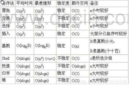
}4. Time and space complexity of common algorithms
Fourth, the space complexity of the algorithm
Similar to the discussion of time complexity, the space complexity (Space Complexity) S(n) of an algorithm is defined as the storage space consumed by the algorithm, which is also a function of the problem size n. Asymptotic space complexity is also often referred to simply as space complexity.
Space Complexity is a measure of the size of the storage space temporarily occupied by an algorithm during its operation. The storage space occupied by an algorithm on the computer memory includes three aspects: the storage space occupied by the storage algorithm itself, the storage space occupied by the input and output data of the algorithm, and the storage space temporarily occupied by the algorithm during its operation. The storage space occupied by the input and output data of the algorithm is determined by the problem to be solved, and is passed from the calling function through the parameter table, which does not change with the algorithm. The storage space occupied by the storage algorithm itself is proportional to the length of the algorithm writing. To compress the storage space in this area, a shorter algorithm must be written. The storage space temporarily occupied by the algorithm during the running process varies with the algorithm. Some algorithms only need to occupy a small amount of temporary work units and do not change with the size of the problem. We call this algorithm "in-place\". Yes, it is a storage-saving algorithm, such as the several algorithms introduced in this section; the number of temporary work units that some algorithms need to occupy is related to the scale n of the problem to be solved, and it increases with the increase of n. , when n is large, it will occupy more storage units, such as the quicksort and mergesort algorithms that will be introduced in Chapter 9.
For example, when the space complexity of an algorithm is a constant, that is, it does not change with the size of the processed data n, it can be expressed as O(1); when the space complexity of an algorithm is the logarithm of n with the base 2 When proportional to , it can be expressed as 0(10g2n); when the complexity of an algorithm is linearly proportional to n, it can be expressed as 0(n). If the formal parameter is an array, you only need to assign a The space for storing an address pointer transmitted by the actual parameter, that is, a machine word space; if the formal parameter is a reference method, it is only necessary to allocate a space for storing an address, and use it to store the address of the corresponding actual parameter variable. , so that the argument variable is automatically referenced by the system.