[OpenCV-Python] 22 Histogram

OpenCV-Python: IV Image Processing in OpenCV

22 Histogram

22.1 Calculation, drawing and analysis of histogram

Goal
　　•Use OpenCV or Numpy function to calculate histogram
　　•Use Opencv or Matplotlib function to draw a histogram
　　•The functions to be learned are: cv2.calcHist(), np.histogram()
principle
　　What is a histogram? Through the histogram, you can have an overall understanding of the gray distribution of the entire image. The x-axis of the histogram is the gray value (0 to 255), and the y-axis is the number of points with the same gray value in the picture.
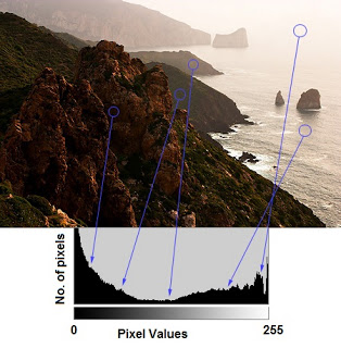
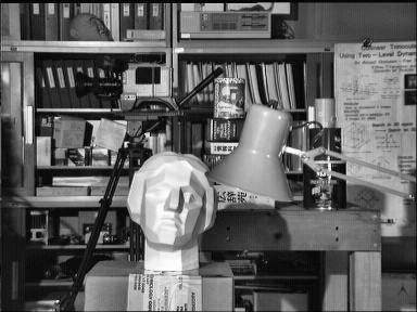
The histogram is actually another interpretation of the image. Take the following picture as an example. Through the histogram, we can have an intuitive understanding of the image's contrast, brightness, and grayscale distribution. Almost all image processing software provides a histogram analysis function. The picture below is from Cambridge in Color website. It is highly recommended that you go to this website to learn more.
Let's take a look at this picture and its histogram together. (Remember that the histogram is drawn based on a grayscale image, not a color image). The left area of ​​the histogram shows the number of darker pixels, and the right side shows the number of brighter pixels. From this picture, you can see that the dark area is larger than the two areas, and there are few pixels in the middle.

22.1.1 Statistical Histogram

Now that we know what a histogram is, how to get a histogram of an image?
　　Both OpenCV and Numpy have built-in functions to do this. Before using these functions, we must want to understand the terminology related to histograms.

BINS: The above histogram shows the number of pixels corresponding to each gray value. If the pixel value is 0 to 255, you need 256 numbers to display the histogram above. However, what if you don't need to know the number of pixels for each pixel value, but only want to know the number of pixels between two pixel values? For example, we want to know the number of pixels with pixel values ​​between 0 and 15, followed by 16 to 31,..., 240 to 255. We only need 16 values ​​to draw the histogram. The content demonstrated by the example in OpenCVTutorials on histograms.
How to do it? You only need to divide the original 256 values ​​into 16 groups and take the sum of each group. And every group here is called BIN. There are 256 BINs in the first example and 16 BINs in the second example. In the OpenCV documentation, use histSize to represent BINS.
DIMS: Indicates the number of parameters that we collect data. In this example, we only consider one thing about the collected data: the gray value. So here is 1.
RANGE: It is the gray value range to be counted, generally speaking [0, 256], that is to say all gray values

Use OpenCV statistical histogram function cv2.calcHist can help us to count the histogram of an image

Can help us to count the histogram of an image. Let's get familiar with this function and its parameters together:
cv2.calcHist(images,channels,mask,histSize,ranges[,hist[,accumulate]])
　　1. images: original image (image format is uint8 or float32). When passing in a function, it should be enclosed in square brackets [], for example: [img].
　　2. channels: also need to be enclosed in square brackets, it will tell the function that we want to count the histogram of that image. If the input image is a grayscale image, its value is [0]; if it is a color image, the incoming parameters can be [0], [1], [2], which correspond to channels B, G, and R respectively.
　　3. mask: mask image. To count the histogram of the entire image, set it to None. But if you want to count the histogram of a certain part of the image, you need to make a mask image and use it. (There are examples below)
　　4. histSize: the number of BINs. It should also be enclosed in square brackets, for example: [256].
　　5. ranges: pixel value range, usually [0, 256]
Let's start with a simple image. Load an image in grayscale format and count the histogram of the image.

img = cv2.imread('home.jpg',0)
# 别忘了中括号 [img],[0],None,[256],[0,256] ，只有 mask 没有中括号
hist = cv2.calcHist([img],[0],None,[256],[0,256])

hist is a 256x1 array, each value represents the number of pixels corresponding to the sub-gray value.

Use Numpy to count histograms. The function np.histogram() in Numpy can also help us count histograms. You can also try the following code:

#img.ravel() 将图像转成一维数组，这里没有中括号。
hist,bins = np.histogram(img.ravel(),256,[0,256])

hist is the same as calculated above. But the bins here are 257, because Numpy calculates
bins in the following ways: 0-0.99, 1-1.99, 2-2.99, etc. So the last range is 255-255.99.
To express it, 256 is added to the end of bins. But we don't need 256, 255 is enough.
Others: Numpy also has a function np.bincount(), which runs ten times faster than np.histgram. So for one-dimensional histograms, we'd better use this function. Don't forget to set minlength=256 when using np.bincount. E.g,

hist=np.bincount(img.ravel() ,minlength=256)
Note: OpenCV function is 40 times faster than np.histgram(). So stick to OpenCV functions.
Now it's time to learn to draw a histogram.

22.1.2 Drawing a histogram

There are two ways to draw a histogram:
　　1. Short Way (simple method): Use the drawing function in Matplotlib.
　　2. Long Way (complex method): Use OpenCV plotting function
Use Matplotlib Matplotlib has a histogram plotting function: matplotlib.pyplot.hist(),
which can directly count and plot histograms. You should use the function calcHist() or np.histogram() to
count the histogram. code show as below:

import cv2
import numpy as np
from matplotlib import pyplot as plt

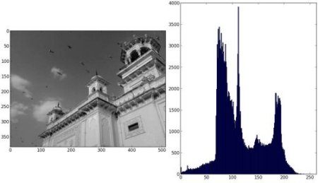
img = cv2.imread('home.jpg',0)
plt.hist(img.ravel(),256,[0,256]); plt.show()

You will get a picture like this:

Or you can just use matplotlib's drawing function, which is useful for drawing multi-channel (BGR) histograms at the same time. But first you have to tell the plotting function where your histogram data is. Run the following code:

import cv2
import numpy as np
from matplotlib import pyplot as plt
img = cv2.imread('home.jpg')
color = ('b','g','r')
# 对一个列表或数组既要遍历索引又要遍历元素时
# 使用内置 enumerrate 函数会有更加直接，优美的做法
#enumerate 会将数组或列表组成一个索引序列。
# 使我们再获取索引和索引内容的时候更加方便
for i,col in enumerate(color):
histr = cv2.calcHist([img],[i],None,[256],[0,256])
plt.plot(histr,color = col)
plt.xlim([0,256])
plt.show()

result:

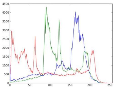
From the histogram above, you can infer that the blue curve is the most on the right side (obviously these are the sky).
Using OpenCV to draw a histogram using OpenCV's own functions is more troublesome. I will not introduce it here. If you are interested, you can study it yourself. You can refer to the official example of OpenCV-Python2.

22.1.3 Using a mask

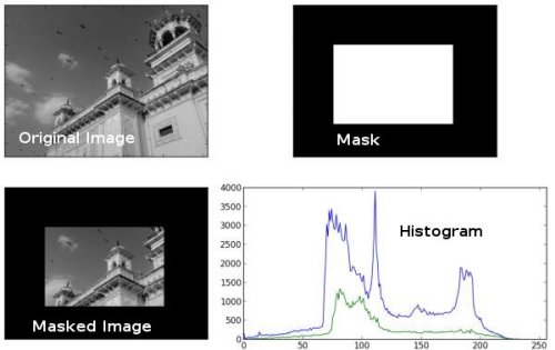
To count the histogram of a certain local area of ​​the image, only a mask image is required. Set the part to be counted as white, and the remaining part as black, which constitutes a mask image. Then pass the mask image to the function.

img = cv2.imread('home.jpg',0)

# create a mask
mask = np.zeros(img.shape[:2], np.uint8)
mask[100:300, 100:400] = 255
masked_img = cv2.bitwise_and(img,img,mask = mask)

# Calculate histogram with mask and without mask
# Check third argument for mask
hist_full = cv2.calcHist([img],[0],None,[256],[0,256])
hist_mask = cv2.calcHist([img],[0],mask,[256],[0,256])

plt.subplot(221), plt.imshow(img, 'gray')
plt.subplot(222), plt.imshow(mask,'gray')
plt.subplot(223), plt.imshow(masked_img, 'gray')
plt.subplot(224), plt.plot(hist_full), plt.plot(hist_mask)
plt.xlim([0,256])

plt.show()

The results are as follows, where the blue line is the histogram of the entire image, and the green line is the histogram after masking.
　　　　

22.2 Histogram equalization

Goal 　　 In
　　this section, we are going to learn the concept of histogram equalization and how to use it to improve the contrast of pictures.

Principle
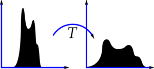
　　Imagine what happens if the pixel values ​​of most pixels in an image are concentrated in one pixel value range? For example, if a picture is very bright as a whole, all the pixel values ​​should be very high. But a high-quality image should have a wide distribution of pixel values. So you should stretch its histogram horizontally (as shown in the figure below). This is what the histogram equalization does. Normally, this operation will improve the contrast of the image.

It is recommended that you read the article on histogram equalization in Wikipedia. The explanation is very powerful. After reading it, I believe you will have a detailed understanding of the whole process. We first look at how to use Numpy to perform histogram equalization, and then learn to use OpenCV to perform histogram equalization.

import cv2
import numpy as np
from matplotlib import pyplot as plt
img = cv2.imread('wiki.jpg',0)
#flatten() 将数组变成一维
hist,bins = np.histogram(img.flatten(),256,[0,256])
# 计算累积分布图
cdf = hist.cumsum()
cdf_normalized = cdf * hist.max()/ cdf.max()
plt.plot(cdf_normalized, color = 'b')
plt.hist(img.flatten(),256,[0,256], color = 'r')
plt.xlim([0,256])
plt.legend(('cdf','histogram'), loc = 'upper left')
plt.show()

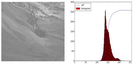
We can see that most of the histogram is in the part with higher gray value, and the distribution is very concentrated. And we hope that the distribution of the histogram is relatively scattered and can cover the entire x-axis. Therefore, we need a transformation function to help us map the current histogram to a widely distributed histogram. This is what the histogram equalization does.
　　We now want to find the minimum value (except 0) in the histogram and use it in the histogram equalization formula in the wiki. But I used Numpy's mask array here. All operations on masked arrays are only valid for non-masked elements. You can go to the Numpy documentation for more information about mask arrays.

# 构建 Numpy 掩模数组， cdf 为原数组，当数组元素为 0 时，掩盖（计算时被忽略）。
cdf_m = np.ma.masked_equal(cdf,0)
cdf_m = (cdf_m - cdf_m.min())*255/(cdf_m.max()-cdf_m.min())
# 对被掩盖的元素赋值，这里赋值为 0
cdf = np.ma.filled(cdf_m,0).astype('uint8')

Now that we have obtained a table, we can know the value of the output pixel corresponding to the input pixel by looking up the table. We only need to apply this transformation to the image.

img2 = cdf[img]

We then draw the histogram and cumulative distribution map according to the previous method, and the results are as follows:

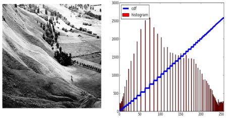
Another important feature is that even if our input picture is a darker picture (unlike the overall bright picture we used above), the same result can be obtained after histogram equalization. Therefore, histogram equalization is often used as a reference tool to make all pictures have the same brightness conditions. This is useful in many situations. For example, for face recognition, before training the classifier, all the pictures in the training set must be histogram equalized to make them reach the same brightness condition.

22.2.1 Histogram equalization in OpenCV

The histogram equalization function in OpenCV is cv2.equalizeHist(). The input image of this function is only a grayscale image, and the output result is the image after the histogram equalization.
The code below still performs histogram equalization on the image above:

img = cv2.imread('wiki.jpg',0)
equ = cv2.equalizeHist(img)
res = np.hstack((img,equ)) #stacking images side-by-side
cv2.imwrite('res.png',res)

Now you can take some photos of different brightness and try it out for yourself. When the data in the histogram is concentrated in a certain gray value range, the histogram equalization is useful. However, if the pixel changes greatly and the grayscale range occupied is very wide, for example, when there are both very bright pixels and very dark pixels. Please see the SOF link in more resources.

22.2.2 CLAHE

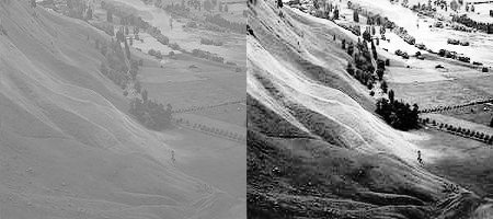
Limited Contrast Adaptive Histogram Equalization The histogram equalization we did above will change the contrast of the entire image, but in many cases, the effect of this is not good. For example, the following figures are the input image and the output image after histogram equalization.

　　Indeed, after the histogram equalization, the contrast of the picture background was changed. But if you compare the faces of the statues in the two images, we have lost a lot of information because of the brightness. The fundamental reason for this result is that the histogram of this image is not concentrated in a certain area (try to draw its histogram, you will understand).
To solve this problem, we need to use adaptive histogram equalization. In this case, the entire image will be divided into many small blocks, these small blocks are called "tiles" (the default size of tiles in OpenCV is 8x8), and then the histogram equalization is performed on each small block ( Similar to the previous).
　　So in each area, the histogram will be concentrated in a small area (unless there is noise interference). If there is noise, the noise will be amplified. In order to avoid this situation, use the contrast limit. For each small block, if the bin in the histogram exceeds the upper limit of contrast, the pixels in it will be evenly distributed to other bins, and then the histogram will be equalized. Finally, in order to remove the "artificial" (due to the algorithm) boundary between each small block, the bilinear difference is used to stitch the small blocks.
The following code shows how to use CLAHE in OpenCV.

import numpy as np
import cv2
img = cv2.imread('tsukuba_l.png',0)
# create a CLAHE object (Arguments are optional).
# 不知道为什么我没好到 createCLAHE 这个模块
clahe = cv2.createCLAHE(clipLimit=2.0, tileGridSize=(8,8))
cl1 = clahe.apply(img)
cv2.imwrite('clahe_2.jpg',cl1)

Here is the result, compare it with the previous result, especially the statue area:

22.3 2D histogram

Goal 　　 In
　　this section we will learn how to draw a 2D histogram, we will use it in the next section.

22.3.1 Introduction

In the previous part, we introduced how to draw a one-dimensional histogram. The reason it is called one-dimensional is because we only consider one feature of the image: the gray value. But in the 2D histogram, we have to consider two image features. For the histogram of color images, we usually need to consider each color (Hue) and saturation (Saturation). Draw a 2D histogram based on these two features.
The official documentation of OpenCV contains an example of creating a color histogram. This section is to learn how to draw color histograms with everyone, which will help us to learn about histogram projection in the next section.

22.3.2 2D histogram in OpenCV

It is simple and convenient to use the function cv2.calcHist() to calculate the histogram. If you want to draw a color histogram, we first need to convert the color space of the image from BGR to HSV. (Remember, to calculate a one-dimensional histogram, you need to convert from BGR to HSV). To calculate a 2D histogram, the parameters of the function need to be modified as follows:
　　• channels=[0 ,1] Because we need to process the H and S channels at the same time.
　　• bins=[180, 256] The H channel is 180, and the S channel is 256.
　　• range=[0, 180, 0, 256] The value of H ranges from 0 to 180, and the value of S ranges from 0 to 256.
code show as below:

import cv2
import numpy as np

img = cv2.imread('home.jpg')
hsv = cv2.cvtColor(img,cv2.COLOR_BGR2HSV)

hist = cv2.calcHist([hsv], [0, 1], None, [180, 256], [0, 180, 0, 256])

That's it, it's easy!

22.3.3 2D Histogram in Numpy

Numpy also provides a function for drawing 2D histograms: np.histogram2d(). (Remember, we used np.histogram() when drawing 1D histograms).

import cv2
import numpy as np
from matplotlib import pyplot as plt

img = cv2.imread('home.jpg')
hsv = cv2.cvtColor(img,cv2.COLOR_BGR2HSV)

hist, xbins, ybins = np.histogram2d(h.ravel(),s.ravel(),[180,256],[[0,180],[0,256]])

The first parameter is the H channel, the second parameter is the S channel, the third parameter is the number of bins, and the fourth parameter is the value range.
Now we are going to see how to draw a color histogram.

22.3.4 Draw 2D Histogram

Method 1: Using cv2.imshow() we get the result is a 180x256 two-dimensional array. So we can use the function cv2.imshow() to display it. But this is a grayscale image. Unless we know the value of the H channel of different colors, we simply don't know what color it represents.
　　Method 2: Use Matplotlib() We can also use the function matplotlib.pyplot.imshow() to draw a 2D histogram, and then match it with a different color map (color_map). In this way, we will have a more intuitive understanding of the value of each point. But like the previous question, you still don't know what the color represents. Nevertheless, I still prefer this method, it is simple and easy to use.
Note: When using this function, remember to set the interpolation parameter to nearest.
code show as below:

import cv2
import numpy as np
from matplotlib import pyplot as plt

img = cv2.imread('home.jpg')
hsv = cv2.cvtColor(img,cv2.COLOR_BGR2HSV)
hist = cv2.calcHist( [hsv], [0, 1], None, [180, 256], [0, 180, 0, 256] )

plt.imshow(hist,interpolation = 'nearest')
plt.show()

Below is the input image and color histogram. The X axis displays the S value, and the Y axis displays the H value.

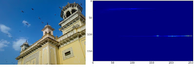
In the histogram, you can see that there are relatively high values ​​near H=100 and S=100. This part corresponds to the blue of the sky. Similarly, another peak is near H=25 and S=100. The yellow color of this palace corresponds. You can modify the image by using image editing software (GIMP), and then draw a histogram to see if I am right.
　　Method 3: OpenCV Grid has an example of color histogram in the official documentation. Run this code, the color histogram you see also shows the corresponding color. Simply put: the output is a histogram coded by color. The effect is very good (although a lot of code has to be added).
In that code, the author first created a color map in HSV format, and then converted it to BGR format. Then multiply the obtained histogram by the color histogram. The author also took a few steps to remove small isolated points, thus getting a good histogram.
I leave the analysis of the code to you, go and play for yourself. The following is the result obtained after running this code on the above graph:

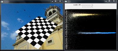
From the histogram, we can clearly see the colors they represent, blue, color change, and white brought by the chessboard, beautiful! ! !

# -*- coding: utf-8 -*-
#!/usr/bin/env python
import numpy as np
import cv2
from time import clock
import sys
import video
#video 模块也是 opencv 官方文档中自带的
if __name__ == '__main__':
    # 构建 HSV 颜色地图
    hsv_map = np.zeros((180, 256, 3), np.uint8)
    # np.indices 可以返回由数组索引构建的新数组。
    # 例如： np.indices （（ 3,2 ））；其中（ 3,2 ）为原来数组的维度：行和列。
    # 返回值首先看输入的参数有几维：（ 3,2 ）有 2 维，所以从输出的结果应该是
    # [[a],[b]], 其中包含两个 3 行， 2 列数组。
    # 第二看每一维的大小，第一维为 3, 所以 a 中的值就 0 到 2 （最大索引数），
    # a 中的每一个值就是它的行索引；同样的方法得到 b （列索引）
    # 结果就是
    # array([[[0, 0],
    # [1, 1],
    # [2, 2]],
    #
    # [[0, 1],
    # [0, 1],
    # [0, 1]]])
    h, s = np.indices(hsv_map.shape[:2])
    hsv_map[:,:,0] = h
    hsv_map[:,:,1] = s
    hsv_map[:,:,2] = 255
    hsv_map = cv2.cvtColor(hsv_map, cv2.COLOR_HSV2BGR)
    cv2.imshow('hsv_map', hsv_map)
    cv2.namedWindow('hist', 0)
    hist_scale = 10
    def set_scale(val):
        global hist_scale
        hist_scale = val
    cv2.createTrackbar('scale', 'hist', hist_scale, 32, set_scale)
    try: fn = sys.argv[1]
    except: fn = 0
    cam = video.create_capture(fn, fallback='synth:bg=../cpp/baboon.jpg:class=chess:noise=0.05')
    while True:
        flag, frame = cam.read()
        cv2.imshow('camera', frame)
        # 图像金字塔
        # 通过图像金字塔降低分辨率，但不会对直方图有太大影响。
        # 但这种低分辨率，可以很好抑制噪声，从而去除孤立的小点对直方图的影响。
        small = cv2.pyrDown(frame)
        hsv = cv2.cvtColor(frame, cv2.COLOR_BGR2HSV)
        # 取 v 通道 ( 亮度 ) 的值。
        # 没有用过这种写法，还是改用最常见的用法。
        #dark = hsv[...,2] < 32
        # 此步操作得到的是一个布尔矩阵，小于 32 的为真，大于 32 的为假。
        dark = hsv[:,:,2] < 32
        hsv[dark] = 0
        h = cv2.calcHist( [hsv], [0, 1], None, [180, 256], [0, 180, 0, 256] )
        #numpy.clip(a, a_min, a_max, out=None)[source]
        #Given an interval, values outside the interval are clipped to the interval edges.
        #For example, if an interval of [0, 1] is specified, values smaller
        #than 0 become 0, and values larger than 1 become 1.
        #>>> a = np.arange(10)
        #>>> np.clip(a, 1, 8)
        #array([1, 1, 2, 3, 4, 5, 6, 7, 8, 8])
        h = np.clip(h*0.005*hist_scale, 0, 1)
        #In numpy one can use the 'newaxis' object in the slicing syntax to create an
        #axis of length one. one can also use None instead of newaxis,
        #the effect is exactly the same
        #h 从一维变成 3 维
        vis = hsv_map*h[:,:,np.newaxis] / 255.0
        cv2.imshow('hist', vis)
        ch = 0xFF & cv2.waitKey(1)
        if ch == 27:
            break
    cv2.destroyAllWindows()

22.4 Histogram back projection

Goal 　　 In
　　this section, we will learn the
principle of
　　histogram back projection. 　　 Histogram back projection is proposed by Michael J. Swain and Dana H. Ballard in their article "Indexing via color histograms".
　　So what is it? It can be used for image segmentation, or to find the part of our interest in the image. Simply put, it will output an image of the same size as the input image (to be searched), and each pixel value in it represents the probability that the corresponding point on the input image belongs to the target object. To explain in simpler words, the higher the pixel value (whiter) the point in the output image, the more likely it is to represent the target we are searching for (where the input image is located). This is an intuitive explanation. Histogram projection is often used together with the camshift algorithm and so on.
How should we implement this algorithm? First we need to create a histogram of an image that contains the target we are looking for (in our example, we are looking for grass, nothing else).
The object we want to find should fill this image as much as possible (in other words, it is best to have and only the object we want to find on this image). It is best to use a color histogram, because the color of an object can be better used for image segmentation and object recognition than its grayscale. Then we project this color histogram into the input image to find our target, that is, to find the probability of the pixel value of each pixel in the input image in the histogram, so that we get a probability image, and finally set Appropriate threshold to binarize the probability image is as simple as that.

22.4.1 Algorithms in Numpy

The algorithm here is slightly different from the algorithm described above.
　　First, we have to create two color histograms, the histogram of the target image ('M'), and (to be searched) the histogram of the input image ('I').

import cv2
import numpy as np
from matplotlib import pyplot as plt

#roi is the object or region of object we need to find
roi = cv2.imread('rose_red.png')
hsv = cv2.cvtColor(roi,cv2.COLOR_BGR2HSV)

#target is the image we search in
target = cv2.imread('rose.png')
hsvt = cv2.cvtColor(target,cv2.COLOR_BGR2HSV)

# Find the histograms using calcHist. Can be done with np.histogram2d also
M = cv2.calcHist([hsv],[0, 1], None, [180, 256], [0, 180, 0, 256] )
I = cv2.calcHist([hsvt],[0, 1], None, [180, 256], [0, 180, 0, 256] )

Calculate the ratio:

back projection R, that is, create a new image based on the "palette" of R, where each pixel represents the probability that this point is the target. For example, B (x,y) =R[h(x,y),s(x,y)], where h is the hue value at point (x,y), and s is the
saturation at point (x,y) value. Finally add another condition .

h,s,v = cv2.split(hsvt)
B = R[h.ravel(),s.ravel()]
B = np.minimum(B,1)
B = B.reshape(hsvt.shape[:2])

Now use a disc operator to do convolution, B = D × B, where D is the convolution kernel.

disc = cv2.getStructuringElement(cv2.MORPH_ELLIPSE,(5,5))
B=cv2.filter2D(B,-1,disc)
B = np.uint8(B)
cv2.normalize(B,B,0,255,cv2.NORM_MINMAX)

Now the largest gray value in the output image is the location of the target we are looking for. If what we are looking for is a region, we can use a threshold to binarize the image, so that we can get a good result.

ret,thresh = cv2.threshold(B,50,255,0)

That's it.

22.4.2 Back projection in OpenCV

The function cv2.calcBackProject() provided by OpenCV can be used to do histogram back projection. Its parameters are basically the same as those of the function cv2.calcHist. One of the parameters is the histogram of the target we want to find. Similarly, before using the target's histogram for back projection, we should first normalize it. The returned result is a probability image. We then use a disc-shaped convolution kernel to perform a volume operation on it, and finally use a threshold for binarization. Here is the code and results:

import cv2
import numpy as np
roi = cv2.imread('tar.jpg')
hsv = cv2.cvtColor(roi,cv2.COLOR_BGR2HSV)
target = cv2.imread('roi.jpg')
hsvt = cv2.cvtColor(target,cv2.COLOR_BGR2HSV)
# calculating object histogram
roihist = cv2.calcHist([hsv],[0, 1], None, [180, 256], [0, 180, 0, 256] )
# normalize histogram and apply backprojection
# 归一化：原始图像，结果图像，映射到结果图像中的最小值，最大值，归一化类型
#cv2.NORM_MINMAX 对数组的所有值进行转化，使它们线性映射到最小值和最大值之间
# 归一化之后的直方图便于显示，归一化之后就成了 0 到 255 之间的数了。
cv2.normalize(roihist,roihist,0,255,cv2.NORM_MINMAX)
dst = cv2.calcBackProject([hsvt],[0,1],roihist,[0,180,0,256],1)
# Now convolute with circular disc
# 此处卷积可以把分散的点连在一起
disc = cv2.getStructuringElement(cv2.MORPH_ELLIPSE,(5,5))
dst=cv2.filter2D(dst,-1,disc)
# threshold and binary AND
ret,thresh = cv2.threshold(dst,50,255,0)
# 别忘了是三通道图像，因此这里使用 merge 变成 3 通道
thresh = cv2.merge((thresh,thresh,thresh))
# 按位操作
res = cv2.bitwise_and(target,thresh)
res = np.hstack((target,thresh,res))
cv2.imwrite('res.jpg',res)
# 显示图像
cv2.imshow('1',res)
cv2.waitKey(0)

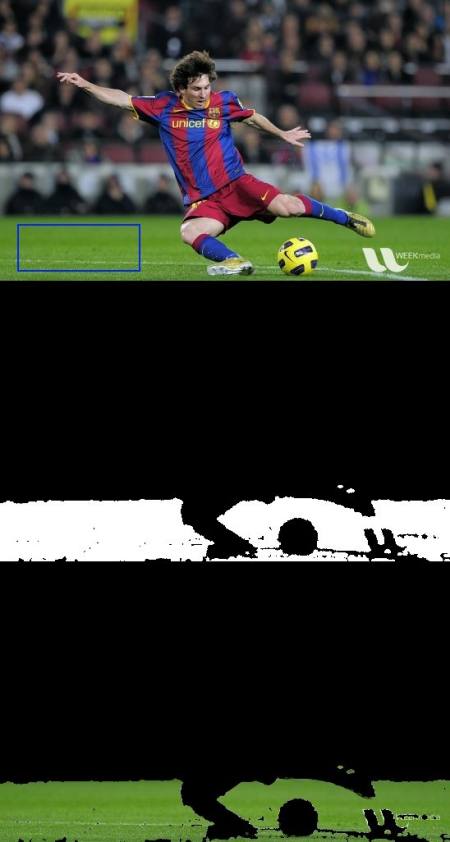
Below is an image I used. I use the area in the blue rectangle in the picture as the sampling object, and then search for all similar areas (grass) in the picture based on this sample.
　　　　

For more information, please pay attention to the official account: