1. Introduction
The TSP problem is the traveling salesman problem. The classic TSP can be described as: a merchandise salesman wants to go to several cities to sell merchandise. The salesman starts from one city and needs to go through all the cities before returning to the place of departure. How should the travel route be chosen to make the total travel the shortest. From the point of view of graph theory, the essence of the problem is to find a Hamiltonian cycle with the smallest weight in a weighted completely undirected graph.
There are many different ways to ask traveling salesman questions. Recently, I have done a few questions about TSP, and I will summarize below. Since most TSP problems are NP-Hard, it is difficult to get any efficient polynomial-level algorithm. Generally, the algorithms used are biased towards brute force search and state pressure DP. Here, state pressure DP is used to solve. The number of locations given by most TSP questions is very small.
Considering the classic TSP problem, if the state pressure DP is used and each location is compressed as binary 1/0, it is not difficult to get the state transition equation:
dp[S][i] = min(dp[S][i] , dp[S ^ (1 << (i-1))][k] + dist[k][i])
S stands for the current state, i (starting from 1) means that the i-th last visited when the current state is reached The locations
k are all locations visited in S that are different from that of i.
dist represents the shortest path between two points.
And initialization:
DP[S][i] = dist[start][i](S == 1<<(i-1))
If you are unfamiliar with the state pressure dp for the first time, please think carefully about the above formula The meaning of this is the key to most TSP problems.
Second, the source code
%%%%%%%%%%%%%%%%%%%%%%%%%初始化%%%%%%%%%%%%%%%%%%%%%%%%%%%%%%%%%
clear all; %清除所有变量
close all; %清图
clc; %清屏
m=50; %蚂蚁个数
Alpha=1; %信息素重要程度参数
Beta=5; %启发式因子重要程度参数
Rho=0.1; %信息素蒸发系数
G_max=200; %最大迭代次数
Q=100; %信息素增加强度系数
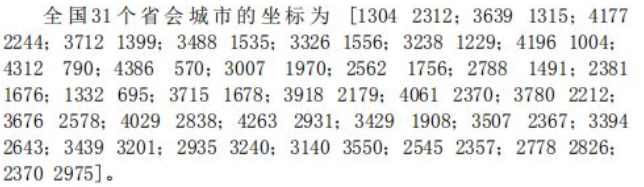
C=[1304 2312;3639 1315;4177 2244;3712 1399;3488 1535;3326 1556;...
3238 1229;4196 1044;4312 790;4386 570;3007 1970;2562 1756;...
2788 1491;2381 1676;1332 695;3715 1678;3918 2179;4061 2370;...
3780 2212;3676 2578;4029 2838;4263 2931;3429 1908;3507 2376;...
3394 2643;3439 3201;2935 3240;3140 3550;2545 2357;2778 2826;...
2370 2975]; %31个省会城市坐标
%%%%%%%%%%%%%%%%%%%%%%%%第一步:变量初始化%%%%%%%%%%%%%%%%%%%%%%%%
n=size(C,1); %n表示问题的规模(城市个数)
D=zeros(n,n); %D表示两个城市距离间隔矩阵
for i=1:n
for j=1:n
if i~=j
D(i,j)=((C(i,1)-C(j,1))^2+(C(i,2)-C(j,2))^2)^0.5;
else
D(i,j)=eps;
end
D(j,i)=D(i,j);
end
end
Eta=1./D; %Eta为启发因子,这里设为距离的倒数
Tau=ones(n,n); %Tau为信息素矩阵
Tabu=zeros(m,n); %存储并记录路径的生成
NC=1; %迭代计数器
R_best=zeros(G_max,n); %各代最佳路线
L_best=inf.*ones(G_max,1); %各代最佳路线的长度
figure(1);%优化解
while NC<=G_max
%%%%%%%%%%%%%%%%%%第二步:将m只蚂蚁放到n个城市上%%%%%%%%%%%%%%%%
Randpos=[];
for i=1:(ceil(m/n))
Randpos=[Randpos,randperm(n)];
end
Tabu(:,1)=(Randpos(1,1:m))';
%%%%%第三步:m只蚂蚁按概率函数选择下一座城市,完成各自的周游%%%%%%
for j=2:n
for i=1:m
visited=Tabu(i,1:(j-1)); %已访问的城市
J=zeros(1,(n-j+1)); %待访问的城市
P=J; %待访问城市的选择概率分布
Jc=1;
for k=1:n
if length(find(visited==k))==0
J(Jc)=k;
Jc=Jc+1;
end
end
%%%%%%%%%%%%%%%%%%计算待选城市的概率分布%%%%%%%%%%%%%%%%
for k=1:length(J)
P(k)=(Tau(visited(end),J(k))^Alpha)...
*(Eta(visited(end),J(k))^Beta);
end
P=P/(sum(P));
%%%%%%%%%%%%%%%%按概率原则选取下一个城市%%%%%%%%%%%%%%%%
Pcum=cumsum(P);
Select=find(Pcum>=rand);
to_visit=J(Select(1));
Tabu(i,j)=to_visit;
end
end
Three, running results


Four, remarks
Complete code or write on behalf of adding QQ1575304183