The Hungarian algorithm was proposed by the Hungarian mathematician Edmonds in 1965, hence the name. The Hungarian algorithm is based on the idea of proof of sufficiency in Hall's theorem. It is the most common algorithm for partial graph matching. The core of the algorithm is to find an augmentation path. It is an algorithm that uses augmentation paths to find the maximum matching of bipartite graphs.
Wiki:
Let G=(V,E) be an undirected graph . For example, the vertex set V can be partitioned into the union of two disjoint subsets V1 and V2, and the two vertices attached to each edge of the graph belong to these two different subsets. Call graph G a bipartite graph . The bipartite graph can also be written as G=(V1,V2,E).
Given a bipartite graph G, in a subgraph M of G, any two edges in the edge set {E} of M are not attached to the same vertex, then M is said to be a match. Choosing the subset with the largest number of edges in such a subset is called the maximum matching problem of the graph (maximal matching problem)
If all the vertices of the graph are associated with an edge in a match, the match is called a complete match , also called a complete , perfect match .
An obvious algorithm for finding the largest match is to find all matches first, and then keep the one with the most matches. But the time complexity of this algorithm is an exponential function of the number of edges. Therefore, a more efficient algorithm is needed. The following introduces the method of using augmented path to find the maximum matching (called the Hungarian algorithm, proposed by mathematician Harold Kuhn in 1955).
Definition of Augmented Road (also called Augmented Track or Staggered Track ):
If P is a path connecting two unmatched vertices in graph G, and the edges belonging to M and edges not belonging to M (that is, the edges that are matched and the edges to be matched) appear alternately on P, then P is called relative to M An augmentation path for (M is a match)
1. The origin and development of ant colony algorithm (ACA)
. In the process of researching new algorithms, Marco Dorigo and others found that when ant colonies are looking for food, they exchange for food by secreting a biological hormone called pheromone. Information can quickly find the target, so in his doctoral thesis in 1991, he first systematically proposed a new intelligent optimization algorithm based on ant population "Ant system (AS)". Later, the proponent and many studies The authors made various improvements to the algorithm and applied it to a wider range of fields, such as coloring problems, secondary allocation problems, workpiece sequencing problems, vehicle routing problems, job shop scheduling problems, network routing problems, large-scale integration Circuit design, etc. In recent years, M. Dorigo and others have further developed the ant algorithm into a general optimization technology "Ant Colony Optimization (ACO)", and called all algorithms that conform to the ACO framework "Ant Colony Optimization Algorithm" ACO algorithm)". 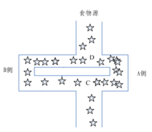
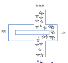
Specifically, each ant started looking for food without prior notification of where the food was. When a person finds food, it will release a volatile secretion pheromone (called pheromone, which will gradually evaporate and disappear over time, and the concentration of pheromone represents the distance of the path). Let other ants perceive and play a guiding role. Generally, when there are pheromone on multiple paths, the ants will give priority to the path with high pheromone concentration, so that the pheromone concentration of the path with high concentration is higher, forming a positive feedback. Some ants do not always repeat the same path like other ants. They will find another way. If the new road is shorter than the original other roads, then gradually, more ants will be attracted to this shorter road. . Finally, after a period of running, there may be a shortest path repeated by most ants. In the end, the path with the highest pheromone concentration is the optimal path ultimately selected by the ants.
Compared with other algorithms, ant colony algorithm is a relatively young algorithm. It has the characteristics of distributed computing, no central control, asynchronous and indirect communication between individuals, and is easy to be combined with other optimization algorithms. After many people with lofty ideals, Exploring, a variety of improved ant colony algorithms have been developed to date, but the principle of ant colony algorithms is still the backbone.
2 The solution principle of the ant colony algorithm
Based on the above description of the foraging behavior of the ant colony, the algorithm mainly simulates the foraging behavior in the following aspects:
1 The simulated picture scene contains two pheromones, one for home, One represents the location of food, and both pheromones are evaporating at a certain rate.
2 Each ant can only perceive information in a small part of its surroundings. When ants are looking for food, if they are within the range of perception, they can go directly. If they are not within the range of perception, they have to move towards a place with a lot of pheromones. There is a small probability that the ant will not go to a place with a lot of pheromones. Taking a different approach, this small probability event is very important, represents a way-finding innovation, and is very important for finding a better solution.
3. The rules for ants returning to their nest are the same as those for finding food.
4. When the ant moves, it will first follow the guidance of the pheromone. If there is no guidance of the pheromone, it will go inertially according to its own moving direction, but there is a certain chance to change the direction. The ant can also remember the way it has traveled. Avoid repeating one place.
5. Ants leave the most pheromones when they find food, and then the farther away from the food, the less pheromone they leave. The rules for finding the amount of pheromone left in the nest are the same as food. Ant colony algorithm has the following characteristics: positive feedback algorithm, concurrency algorithm, strong robustness, probabilistic global search, not relying on strict mathematical properties, long search time, and easy to stop.
The ant transition probability formula: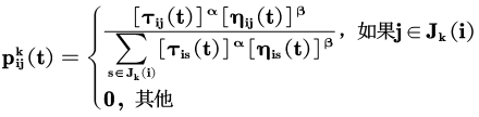
In the formula: is the probability of ant k transferring from city i to j; α and β are the relative importance of pheromone and heuristic factor respectively; is the amount of pheromone on the edge (i, j); is the heuristic factor; is The next step allows Ant to select the city. The above formula is the pheromone update formula in the ant system, which is the amount of pheromone on the edge (i, j); ρ is the pheromone evaporation coefficient, 0<ρ<1; is the kth ant staying in this iteration The amount of pheromone on the edge (i, j); Q is a normal coefficient; it is the path length of the kth ant in this trip.
In the ant system, the pheromone update formula is: 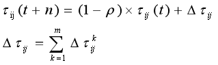
3 Solving steps of the ant colony algorithm :
1. Initialization parameters At the beginning of the calculation, relevant parameters need to be initialized, such as ant colony size (number of ants) m, pheromone importance factor α, heuristic function importance factor β, pheromone will generate silver ρ, total pheromone release Q, maximum number of iterations iter_max, initial number of iterations iter=1.
1. Construct the solution space and place each ant randomly at a different starting point. For each ant k (k=1,2,3...m), calculate the next city to be visited according to (2-1) until all ants After visiting all cities.
2. Update information Su calculate the length of each ant's path Lk (k=1,2,...,m), and record the optimal solution (shortest path) in the current iteration times. At the same time, the pheromone concentration on the connection path of each city is updated according to formulas (2-2) and (2-3).
3. Determine whether to terminate. If iter<iter_max, set iter=iter+1, clear the record table of the ant's path, and return to step 2; otherwise, terminate the calculation and output the optimal solution.
4. Determine whether to terminate. If iter<iter_max, set iter=iter+1, clear the record table of the ant's path, and return to step 2; otherwise, terminate the calculation and output the optimal solution. 3. Determine whether to terminate. If iter<iter_max, set iter=iter+1, clear the record table of the ant's path, and return to step 2; otherwise, terminate the calculation and output the optimal solution. 
4 Simple case-steps based on ant colony algorithmSolve the minimum value of the binary function to optimize the binary function:
(4-1) Optimization idea: First, by solving the constraints, we can get the search space composed of feasible solutions that meet the constraints. This is a two-dimensional convex space. If the range search of each component is equally divided into discrete points, then the entire size of the space can be determined by the division thickness of the component xi. Assuming that xi is divided into Ni parts, there are 2*Ni in the entire search space. Moreover, in order to obtain an accurate solution, the interval of the component xi is divided very finely, then the search space will become very large, which is the difficulty of solving the problem. Of course, this method of dividing the interval is also commonly used by many optimization algorithms. method. ) Divide the value interval of each component equally into N points, then xi has N choices of two-dimensional decision variables x has N^2 choice combinations. And consider the N value points of each component as N cities. At the beginning, m Ants are randomly placed on m Cities in N of x1. After the search starts, Ant selects the city according to the transition probability. In the first selection, use the rand function to select randomly, and then transfer according to the selection probability.
The specific steps of this case are: (1) Solve the constraint conditions to obtain the interval of each component, which is known from the question [-1,1]; (2) Refine the component interval to establish a search space, and this case is subdivided into 73 Xi=[-1,-1+2/73,…1]; (3) Determine whether the accuracy meets the requirements, if it is satisfied, output the optimal solution and end, otherwise continue (4); (4) each Set the initial value of the amount of information on the path; (5) Randomly select the path to solve; (6) Each ant chooses the path to solve according to the selection probability;
(7) If each ant finds the solution, continue (8), otherwise go to ( 4); (8) Refine the components of the current optimal solution and turn to (2).
clc;
clear;
%% initialization

% Define the position of the robots
% % Robot_position=[1,2;1,4;1,6;1,8;1,10];
% Robot_position=[5,7;3,2;7,13;6,9;5,5];
% % Define the target positions
% Target_position=[3,6;5,4;5,6;5,8;8,6];

% Random position
UAV_number=2; % The number of UAVs
task_number=5; % The number of Target positions
SizeofMap = [1 100];
size_UAV = 0;
size_task = 0;

while (size_UAV<UAV_number && size_task < task_number)
    UAV_position = randi(SizeofMap,UAV_number,2);
    Target_position = randi(SizeofMap,task_number,2);
    % UAV_position = unique(UAV_position,'rows');
    % Target_position = unique(Target_position,'rows');
    size_UAV = size(unique(UAV_position,'rows'),1);
    size_task = size(unique(Target_position,'rows'),1);
end

% Initial the speed of UAVs
UAV_speed=ones(UAV_number,1)*50;


% UAV_position = randi([1,15],10,2);
% Target_position = randi([1,15],10,2);

% UAV_number=5; % The number of UAVs
% task_number=5; % The number of Target positions
maxT=10; % The maximum tasks can be done by a single worker
task_fixed_number=1; % The number of workers are required for a single task
% unfinishtask_number=task_number;

ant_num_TA=50; % The numbder of ants in Task Allocation
ant_num_PP=30; % The numbder of ants in Path Planning
iteratornum_TA=30; % The iteration times in Task Allocation
iteratornum_PP=10; % The iteration times in Path Planning


% pheromoneMatrix = [];% The matrix to store the pheromone
% maxPheromoneMatrix = []; % The assigned workers based on the pheromone matrix
% criticalPointMatrix = [];% This matrix is used to decide allocation by
% % using pheromone matrix or randomly
%
% % Initialize the last 3 matrix
% % The pheromone are initialized as all '1'
% pheromoneMatrix = ones(task_number,UAV_number);
% for i=1:task_number
%     % From beginning, assign the workers randomly
%     maxPheromoneMatrix(i) =unidrnd(UAV_number) ;
%     % Once the value less or equal to 1, the allocation is based on the
%     % pheromone matrix; otherwise, it is allocated randomly. For
%     % initialization, the tasks are allocated randomly.
%     criticalPointMatrix(i)=ceil(ant_num/task_number );
% end

%% The implementation of Ant Colony Algorithm


%task_number =  task_number_new;
tic;
best_ant_path = AntColonyTaskAllocation(UAV_position,Target_position,UAV_number,UAV_speed,task_number,...
    ant_num_TA, iteratornum_TA, maxT,task_fixed_number, ant_num_PP, iteratornum_PP);
toc;

[row,col]=find(best_ant_path==1);

for i = 1: UAV_number
    mid = find(col==i);
    possibility(i) =length(mid);
end
%
%         task_number_imme = task_number;
Best_Strategy_entire = zeros( max(possibility),UAV_number);
for i = 1: UAV_number
    mid = find(col==i);
    for j = 1: length(mid)
        Best_Strategy_entire(j,i)=row(mid(j));
    end
end


%%  Display the task allcocation strategy

count = ones(1,UAV_number); % count which task the UAV is handling
while (isempty (Target_position) == 0)

    for i = 1: UAV_number
        Best_Strategy(1,i) = Best_Strategy_entire(count(i),i);
    end

    for j = 1:size(Best_Strategy,2)
        if(Best_Strategy(1,j) == 0)
            %Best_Strategy_updated(i,j)=0;
            %Target_position(Best_Strategy(1,j),:) = UAV_position( j, :);
            UAV_step(j,:)=[0, 0];
            %task_number=task_number+1;
        else
            %     end

            %     for j =1: size(Best_Strategy,2)
            difference(j,:)=Target_position(Best_Strategy(j),:)-UAV_position(j,:);
            if (difference(j,1)==0)
                angle(j)= pi/2;
            else
                angle(j)= atan(difference(j,2)/difference(j,1));
            end
            %     end
            %end

            % for i= 1: size(Best_Strategy,1)
            %     for j= 1: size(Best_Strategy,2)
            if (difference(j,1) > 0)
                UAV_step(j,1)= UAV_speed(j)*cos(angle(j));
                UAV_step(j,2)= UAV_speed(j)*sin(angle(j));
            elseif(difference(j,1) < 0)
                UAV_step(j,1)= -UAV_speed(j)*cos(angle(j));
                UAV_step(j,2)= -UAV_speed(j)*sin(angle(j));
            elseif ((difference(j,1) == 0)&& (difference(j,2) > 0))
                UAV_step(j,1)= UAV_speed(j)*cos(angle(j));
                UAV_step(j,2)= UAV_speed(j)*sin(angle(j));
            elseif ((difference(j,1) == 0)&& (difference(j,2) < 0))
                UAV_step(j,1)= - UAV_speed(j)*cos(angle(j));
                UAV_step(j,2)= - UAV_speed(j)*sin(angle(j));
            end
        end
    end

    [UAV_position_new,Target_position_new,task_number, count] = Draw_Strategy(UAV_position,Target_position,...
        Best_Strategy, SizeofMap, UAV_step, UAV_speed, task_number, count);
    if (task_number == 0)
        break;
Complete code or write on behalf of adding QQ1575304183