Linear regression forecasting sales-lasso/ridge model

ElasticNet: A combination of L1 regularization and L2 regularization.
https://blog.csdn.net/weixin_42567027/article/details/107450610

Model introduction

lasso is L1 regularization, the absolute value of the penalty coefficient, each coefficient is contracted after penalty, and it has variable selection function.
ridge is L2 regularization, the square of the penalty coefficient, after penalty, some coefficients directly become 0, and other coefficients shrink.

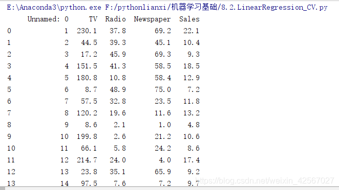
data set

Insert picture description here
Code

// An highlighted block
import numpy as np
import matplotlib as mpl
import matplotlib.pyplot as plt
import pandas as pd
#数据分割为训练数据和测试数据
from sklearn.model_selection import train_test_split
#使用lasso，ridge模型
from sklearn.linear_model import Lasso, Ridge
#交叉验证
from sklearn.model_selection import GridSearchCV


if __name__ == "__main__":

    '''加载数据'''
    # 数据读入
    data = pd.read_csv('F:\pythonlianxi\Advertising.csv')    # TV、Radio、Newspaper、Sales
    #print(data)
    #训练数据
    x = data[['TV', 'Radio', 'Newspaper']]
    # x = data[['TV', 'Radio']]
    #标签集
    y = data['Sales']
    # print(x)
    # print (y)

    '''训练模型'''
    #将数据分割为实验数据，测试数据
    #train_size(0.75)  或者  train_size(100)
    x_train, x_test, y_train, y_test = train_test_split(x, y, random_state=1)
    #建立lasso模型
    model = Lasso()
    #model = Ridge()
    # 模型参数alpha：创建等比数列
    alpha_can = np.logspace(-3, 2, 10)
    #默认小数会以科学计数法的形式输出
    np.set_printoptions(suppress=True)
    #print ('alpha_can = ', alpha_can)  cv=5 :五折交叉验证
    #训练模型
    lasso_model = GridSearchCV(model, param_grid={
    
    'alpha': alpha_can}, cv=5)

    print(u'开始建模...')
    #拟合模型，调参
    lasso_model.fit(x_train, y_train)
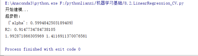
    print( '超参数：\n', lasso_model.best_params_)
    #测试数据做递增排序
    order = y_test.argsort(axis=0)
    y_test = y_test.values[order]
    x_test = x_test.values[order, :]
    #使用测试数据测试模型
    y_hat = lasso_model.predict(x_test)

    '''计算R2，MSE'''
    #r2
    r2=(lasso_model.score(x_test, y_test))
    mse = np.average((y_hat - np.array(y_test)) ** 2)  # Mean Squared Error
    rmse = np.sqrt(mse)  # Root Mean Squared Error
    print('R2:', r2)
    print(mse,rmse)
    # t：样本标号
    t = np.arange(len(x_test))

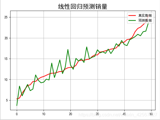
    '''绘图'''
    mpl.rcParams['font.sans-serif'] = [u'simHei']
    mpl.rcParams['axes.unicode_minus'] = False
    plt.figure(facecolor='w')
    plt.plot(t, y_test, 'r-', linewidth=2, label=u'真实数据')
    plt.plot(t, y_hat, 'g-', linewidth=2, label=u'预测数据')
    plt.title(u'线性回归预测销量', fontsize=18)
    plt.legend(loc='upper right')
    plt.grid()
    plt.show()

Experimental results

Insert picture description here