1. Introduction
Single-layer feedforward neural network (SLFN) has been widely used in many fields due to its good learning ability. However, the inherent shortcomings of traditional learning algorithms, such as BP, have become the main bottleneck restricting their development. Feedforward neural networks Most of them use the gradient descent method, which has the following shortcomings and shortcomings:
1. The training speed is slow. Since the gradient descent method requires multiple iterations to achieve the purpose of correcting the weights and thresholds, the training process takes a long time;
2. It is easy to fall into a local minimum and cannot reach the global minimum;
3. The choice of learning rate yita is sensitive. The learning rate has a greater impact on the performance of the neural network. You must choose a suitable one to achieve a more ideal effect. If it is too small, the algorithm will converge slowly, and the training process will take a long time and too large , The training process may be unstable.
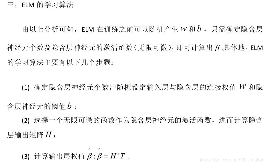
This article will introduce a new SLFN algorithm, the extreme learning machine, which will randomly generate the connection weights between the input layer and the hidden layer and the threshold of the hidden layer neurons, and there is no need to adjust during the training process, just By setting the number of neurons in the hidden layer, the only optimal solution can be obtained. Compared with the traditional training method, this method has the advantages of fast learning rate and good generalization performance.
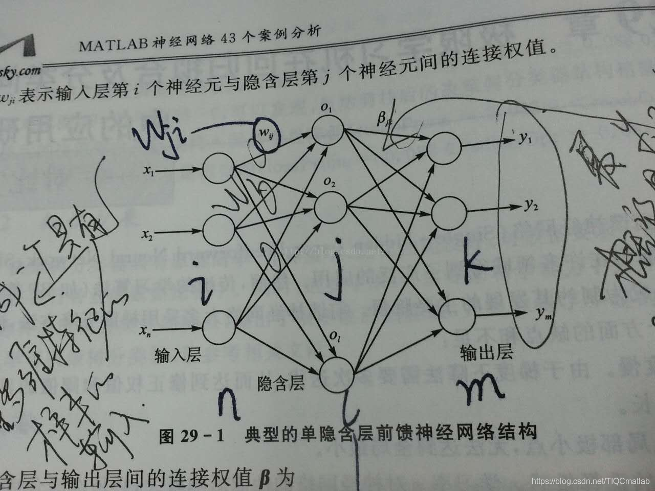
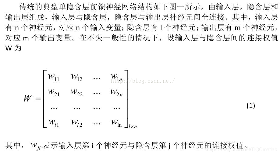
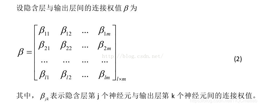
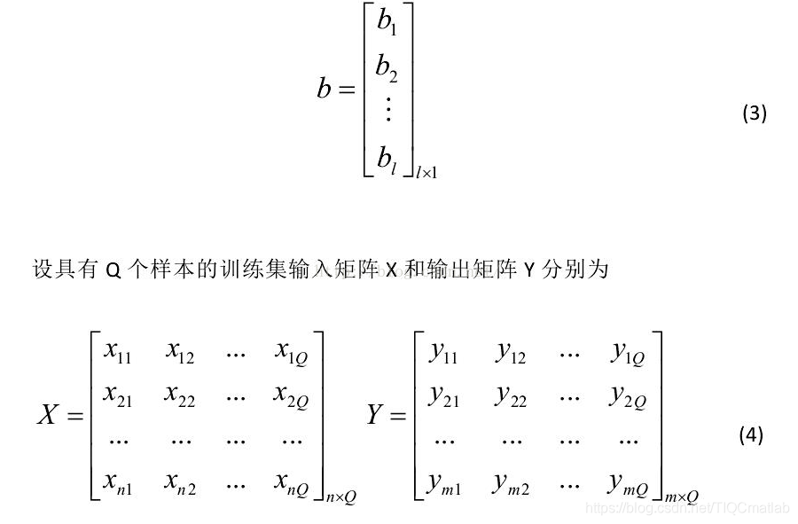
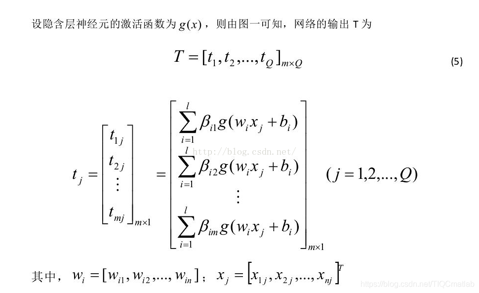
A typical single hidden layer feedforward neural network is shown in the figure above. The input layer and hidden layer, and the hidden layer and output layer are fully connected. The number of neurons in the input layer is determined according to the number of samples and the number of features, and the number of neurons in the output layer is determined according to the number of types of samples.

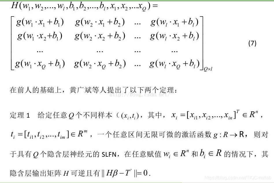
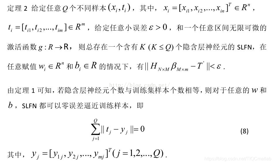
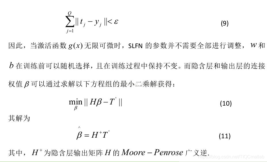
When the number of hidden layer neurons is the same as the number of samples, Eq. (10) has a unique solution, which means that the training samples are approximated with zero error. In the usual learning algorithm, W and b need to be adjusted continuously, but the research results tell us that they do not need to be adjusted continuously, and can even be specified at will. Adjusting them is not only time-consuming, but also not much benefit. (There are doubts here, which may be taken out of context, and this conclusion may be based on a certain premise).


To sum up: ELM and BP are both based on the architecture of feedforward neural network. Their difference lies in the different learning methods. BP uses the gradient descent method to learn by back propagation, which requires continuous Iteratively update the weights and thresholds, while ELM achieves the purpose of learning by increasing the number of hidden layer nodes. The number of hidden layer nodes is generally determined according to the number of samples, and the hidden layer The number is related to the number of samples. In fact, in many forward neural networks, the default maximum number of hidden layer nodes is the number of samples (such as RBF). It does not require iteration, so the speed is much faster than BP. The essence of ELM lies in the two theorems he relies on, these theorems determine his learning style. The weight w between the input layer and the hidden layer and the threshold b of the hidden layer node are obtained through random initialization and do not need to be adjusted. Generally, the number of hidden layer nodes is the same as the number of samples (when the number of samples is relatively small).
The matlab code of ELM can be downloaded directly on the Internet, and the principle is very simple. The process of ELMtrain is to calculate the weight between the hidden layer and the output layer. It is obtained by formula 11 according to the label matrix T. ELMpredict uses the hidden The weight between the containing layer and the output layer is used to calculate the output T. Of course, the weight between the randomly initialized input node and the hidden layer node and the threshold value of the hidden layer node in the ELMtrain will be copied, and no random initialization will be performed. (Otherwise, the weights between the hidden layer and the output layer are calculated in vain, because they are calculated based on the values initialized randomly in ELMtrain) So the entire extreme learning machine is still very simple.
Extreme learning machine is a way of learning, deep learning can also be combined with extreme learning machine, such as ELM-AE
The extreme learning machine has the same idea as the radial basis neural network. By increasing the number of hidden layer neurons, it is possible to map the linearly inseparable samples to the high-level linearly separable space, and then pass between the hidden layer and the output layer. Linear division to complete the classification function, but the activation function of the radial basis is the radial basis function used, which is equivalent to the kernel function in svm (radial basis kernel function)
After reading the RBF neural network, I found that the extreme learning machine must be affected by the idea of RBF. Because RBF also has as many hidden layer nodes as possible, and the strict radial basis network requires that the number of hidden layer nodes is equal to the number of input samples, and the hidden layer neurons and the output layer neurons are also linearly weighted. The final output, the weight between the hidden layer and the output layer, RBF is obtained by solving the linear equation, and the extreme learning machine is also obtained by solving the linear equation through the generalized inverse matrix output by the hidden layer.
Theorem one is the regularized RN (universal approximator) in the corresponding RBF, that is, the number of hidden layer nodes = the number of input samples, the theorem two is the generalized network GN (pattern classifier) in the corresponding RBF, the hidden layer Node <the number of input samples, personally feel that the extreme learning machine is a combination of the learning ideas of RBF and BP algorithms. The input layer and the hidden layer are BP, and the hidden layer and the output layer are RBF. Of course, the hidden layer node The number is also used in two forms of RBF, namely RN and GN.
Second, the source code
function [time, Et]=ANFISELMELM(adaptive_mode)
adaptive_mode = 'none';
tic;
clc;
clearvars -except adaptive_mode;
close all;
% load dataset
data = csvread('iris.csv');
input_data = data(:, 1:end-1);
output_data = data(:, end);
% Parameter initialization
[center,U] = fcm(input_data, 3, [2 100 1e-6]); %center = center cluster, U = membership level
[total_examples, total_features] = size(input_data);
class = 3; % [Changeable]
epoch = 0;
epochmax = 400; % [Changeable]
%Et = zeros(epochmax, 1);
[Yy, Ii] = max(U); % Yy = max value between both membership function, Ii = the class corresponding to the max value
% Population initialization
pop_size = 10;
population = zeros(pop_size, 3, class, total_features); % parameter: population size * 6 * total classes * total features
velocity = zeros(pop_size, 3, class, total_features); % velocity matrix of an iteration
c1 = 1.2;
c2 = 1.2;
original_c1 = c1;
original_c2 = c2;
r1 = 0.4;
r2 = 0.6;
max_c1c2 = 2;
% adaptive c1 c2
% adaptive_mode = 'none';
% class(adaptive_mode)
iteration_tolerance = 50;
iteration_counter = 0;
change_tolerance = 10;
is_first_on = 1;
is_trapped = 0;
%out_success = 0;
for particle=1:pop_size
a = zeros(class, total_features);
b = repmat(2, class, total_features);
c = zeros(class, total_features);
for k =1:class
for i = 1:total_features % looping for all features
% premise parameter: a
aTemp = (max(input_data(:, i))-min(input_data(:, i)))/(2*sum(Ii' == k)-2);
aLower = aTemp*0.5;
aUpper = aTemp*1.5;
a(k, i) = (aUpper-aLower).*rand()+aLower;
%premise parameter: c
dcc = (2.1-1.9).*rand()+1.9;
cLower = center(k,total_features)-dcc/2;
cUpper = center(k,total_features)+dcc/2;
c(k,i) = (cUpper-cLower).*rand()+cLower;
end
end
population(particle, 1, :, :) = a;
population(particle, 2, :, :) = b;
population(particle, 3, :, :) = c;
end
%inisialisasi pBest
pBest_fitness = repmat(100, pop_size, 1);
pBest_position = zeros(pop_size, 3, class, total_features);
% calculate fitness function
for i=1:pop_size
particle_position = squeeze(population(i, :, :, :));
e = get_fitness(particle_position, class, input_data, output_data);
if e < pBest_fitness(i)
pBest_fitness(i) = e;
pBest_position(i, :, :, :) = particle_position;
end
end
% find gBest
[gBest_fitness, idx] = min(pBest_fitness);
gBest_position = squeeze(pBest_position(idx, :, :, :));
% ITERATION
while epoch < epochmax
epoch = epoch + 1;
% calculate velocity and update particle
% vi(t + 1) = wvi(t) + c1r1(pbi(t) - pi(t)) + c2r2(pg(t) - pi(t))
% pi(t + 1) = pi(t) + vi(t + 1)
r1 = rand();
r2 = rand();
for i=1:pop_size
velocity(i, :, :, :) = squeeze(velocity(i, :, :, :)) + ((c1 * r1) .* (squeeze(pBest_position(i, :, :, :)) - squeeze(population(i, :, :, :)))) + ((c2 * r2) .* (gBest_position(:, :, :) - squeeze(population(i, :, :, :))));
population(i, :, :, :) = population(i, :, :, :) + velocity(i ,:, :, :);
end
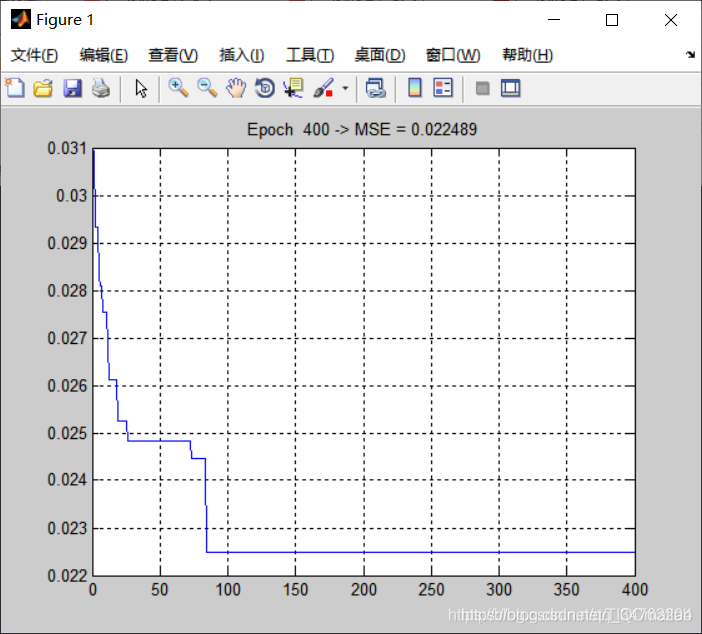
% Draw the SSE plot
plot(1:epoch, Et);
title(['Epoch ' int2str(epoch) ' -> MSE = ' num2str(Et(epoch))]);
grid
pause(0.001);
end
%[out output out-output]
% ----------------------------------------------------------------
time = toc;
end
Three, running results
Four, remarks
Complete code or writing add QQ2449341593 past review
>>>>>>
[Mathematical modeling] Matlab SEIRS infectious disease model [including Matlab source code 033]
[Mathematical modeling] Matlab cellular automata based population evacuation simulation [ Including Matlab source code 035]