Reduce losses
Iterative method
ILC may make you think of "Hot and Cold" This finding hidden items (such as thimble) children's games. In our game, "hidden items" is the best model. At first, you will be wild speculation ( "w1 value of 0."), wait for the system tells you how much loss. Then, you try another guess ( "w1 is 0.5."), To see how much loss. Oh, this time closer to the goal. In fact, if you play the game the right way, often getting close to the target. This game is really tough place to find the best model as efficiently as possible .

Figure 1 . Iterative method for training model.
We will use the same method throughout the iterative machine learning crash course in detail a variety of complex situations, especially in the blue region of the storm cloud. Iteration strategy used in machine learning is very common, mainly because they can be a good scale to large data sets .
"Model" section, one or more features as input, and returns a prediction (y ') as an output. For simplicity, consider a feature of using one kind of a prediction model and returns:
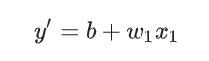
We should b and W1 which initial value? For linear regression problem, the fact that the initial value is not important. We can randomly select a value, but we chose to adopt the following values irrelevant:
- b=0
- W1 = 0
assuming a first characteristic value is 10. The characteristic values are substituted into the prediction function will get the following results:
  y' = 0 + 0(10)
  y' = 0
Figure "Calculated loss" section is to be used to model loss function . Suppose we use the quadratic loss function . Loss of function takes two input values:
- Model predictive feature of x: y '
- y: x corresponding to the correct feature tag
Finally, we look at FIG. "Calculating parameter update" section. Machine learning system in this section is to check the value of the loss function, and of b and W1 generate new values. Now, assume that the mysterious green block produces a new value, then the machine learning system will re-evaluate all features from all labels, generates a new value for the loss function, which in turn produces a new value parameter. This learning process will continue iterated until the algorithm discovered the loss of the lowest possible model parameters . Typically, you can continue to iterate until the total loss will not change, or at least change very slowly so far. At this time, we can say that the model has been convergence .
Gradient descent
FIG iterative method ( FIG. 1 ) contains a title "calculation parameter update" slick green box. Now, we will replace this flashy algorithm more substantial way.
Suppose we have the time and computational resources to calculate W1 all the possible loss of value. We have been for loss and regression study, produced by W1 graphic is always male. In other words, FIG bowl pattern is always as follows:


Then, gradient descent algorithm calculates the gradient at the beginning of the loss curve. In short, the gradient is the vector of partial derivatives; it can let you know which direction from the target "closer" or "farther." Please note that the loss of weight relative to the weight of a single gradient (FIG. 3) is equal to the derivative.
Please note, the gradient is a vector thus has the following two characteristics:
- direction
- size
gradient always refers to the loss of function of the most rapid growth direction. Gradient descent algorithm will take a step in the direction of the negative gradient, in order to reduce losses as soon as possible.


Then, gradient descent will repeat this process, gradually approaching the lowest point .
Learning rate
As stated earlier, the gradient vector having a direction and a magnitude. Gradient descent algorithm with a gradient of a scalar multiplied called a learning rate (also sometimes referred to as step size) to determine the position of the next point. For example, if the gradient magnitude is 2.5, learning rate is 0.01, the gradient descent algorithm selects from 0.025 previous point as the next point location.
Ultra parameter is used to adjust the knob programmer in machine learning algorithm. Most machine learning programmers will spend quite a bit of time to adjust learning rate. If you choose the learning rate is too small, it will take too long to learn:


