(BGV12)同态加密方案初学

BGV主要优化了BV11中的维度-模约减技术，提出了模交换技术，同时也优化了重线性化技术，提出了密钥交换技术，使得无需Bootstrapping也能做到较多层数的同态乘法。

前置

另一种形势的LWE公钥加密

这里在介绍方案的时候采用的另一种形式的LWE公钥加密，不是原文中的内容，但是有必要提一下，不然对于小白会懵逼很久（比如我）。
实例依然是$As+e$

1. $KenGen()$：公钥$pk=\left[\begin{array}{c}-A\\ sA+2e\end{array}\right]$，私钥$sk=[s,1]$，使得$sk\cdot pk=2e$（矩阵乘法即可验证）

2. $Enc()$：$En{c}_{pk}(m)=pk\cdot r+\left[\begin{array}{c}⋮\\ 0\\ m\end{array}\right](\mathrm{m}\mathrm{o}\mathrm{d}q)$，其中$r$均匀取自 { 0 , 1 } L \{0,1\}^L { 0,1}L，是个只含0和1的列矩阵，消息 m ∈ { 0 , 1 } m \in \{0,1\} m∈{ 0,1}

3. $Dec()$：$De{c}_{sk}(ct)=<sk,ct>\mathrm{m}\mathrm{o}\mathrm{d}2$
   可以解密验证一下
   $$\begin{array}{rl}<sk,ct>& =sk\cdot (pk\cdot r+\left[\begin{array}{c}⋮\\ 0\\ m\end{array}\right])\\ & =sk\cdot pk\cdot r+sk\left[\begin{array}{c}⋮\\ 0\\ m\end{array}\right]\\ & =<2e,r>+m\\ & \approx m\end{array}$$
   （$<,>$这个是内积。）
   文章中把$[<\mathbf{c},\mathbf{s}>{]}_q$称为密钥$\mathbf{s}$下密文$c$的噪声

同态加法和乘法构建

接下来根据上面的来试着构建一下密文加法和乘法。
设两个密文${\mathbf{c}}_1,{\mathbf{c}}_2$，满足$<{\mathbf{c}}_1,\mathbf{s}>=2e_1+m_1,<{\mathbf{c}}_2,\mathbf{s}>=2e_2+m_2$
有些地方省略了一下但是默认要模$q$

• 加法
  想构造出明文消息相加的形式，比较简单
  $${\mathbf{c}}_{add}=<{\mathbf{c}}_1+{\mathbf{c}}_2>\mathrm{m}\mathrm{o}\mathrm{d}q$$
  解密：
  $$\begin{array}{rl}Dec({\mathbf{c}}_{add})& =<{\mathbf{c}}_{add},\mathbf{s}>\\ & =<{\mathbf{c}}_1+{\mathbf{c}}_2,\mathbf{s}>\\ & =<{\mathbf{c}}_1,\mathbf{s}>+<{\mathbf{c}}_2,\mathbf{s}>\\ & =m_1+m_2+noise\end{array}$$
  显然符合同态加法。
• 乘法
  想构造出两个密文的乘积解密后是两个明文乘积的样子。
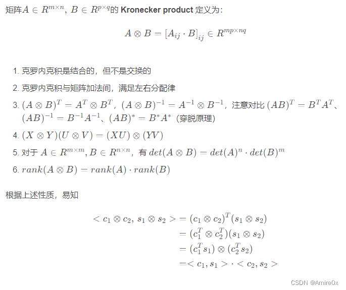
  这里BGV方案中作者观察到
  $$<{\mathbf{c}}_1,\mathbf{s}>\cdot <{\mathbf{c}}_2,\mathbf{s}>=<{\mathbf{c}}_1\otimes {\mathbf{c}}_2,\mathbf{s}\otimes \mathbf{s}>$$
  （$\otimes$这个是张量积），上面的等式可以通过把左边的每一项拆开计算，比如把$c$和$s$都看二维的，计算左边表达式的结果，然后把所有的$c$和$s$分开成内积的形式，就能得到这个结果。
  事实上这个来源于克罗内克积
  
  解密：
  $$\begin{array}{rl}Dec({\mathbf{c}}_{mult})& =<{\mathbf{c}}_1\otimes {\mathbf{c}}_2,\mathbf{s}\otimes \mathbf{s}>\\ & =<{\mathbf{c}}_1,\mathbf{s}>\cdot <{\mathbf{c}}_2,\mathbf{s}>\\ & =(2e_1+m_1)(2e_2+m_2)\\ & =m_1{m}_2+noise\end{array}$$

因此，定义的同态操作如下：
$$\begin{array}{l}Addition:\mathrm{Dec}\left(c_1+c_2,s\right)=\mathrm{Dec}\left(c_1,s\right)+\mathrm{Dec}\left(c_2,s\right)\\ \\ Multplication:\mathrm{Dec}\left(c_1\otimes c_2,s\otimes s\right)=\mathrm{Dec}\left(c_1,s\right)\cdot \mathrm{Dec}\left(c_2,s\right)\end{array}$$
同时我们可以看到，由于乘法定义为了张量积，那么密文和私钥就会膨胀得很厉害，所以需要降低它们。

GLWE（General Learning with Errors）

在BGV方案中把LWE和RLWE统一成了GLWE。
LWE中实例为$(a,b)\leftarrow {\mathbb{Z}}_q^n\times {\mathbb{Z}}_q$
RLWE中的实例为$(a_i,b_i)\leftarrow R_q\times R_q$
如果把$\mathbb{Z}$也看做环，那么即可将二者统一起来。
GLWE的定义如下，

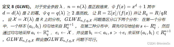
则，可以通过两个参数(d,n)来确定选择的是LWE还是RLWE，LWE 只是用 d = 1 实例化的 GLWE。RLWE 是用 n = 1 实例化的 GLWE。
总之这不是一个新的结构，实际使用的还是RLWE和LWE。

基本方案

• $\mathsf{E}.\mathsf{S}\mathsf{e}\mathsf{t}\mathsf{u}\mathsf{p}(1^{\lambda },1^{\mu },b)$: 由比特$b$来确定我们是构造LWE假设下的方案($b=0$)还是RLWE假设下的方案($b=1$). 选择一个$\mu$比特的模数$q$和参数
  $$d=d(\lambda ,\mu ,b),n=n(\lambda ,\mu ,b),N=\lceil (2n+1)\log q\rceil ,\chi =\chi (\lambda ,\mu ,b)$$
  此处要求最终的参数使得GLWE问题实例具有$2^{\lambda }$强度. 令$R=\mathbb{Z}[x]/(x^d+1)$, 并令参数集合$params=(q,d,n,N,\chi )$.

• $\mathsf{E}.\mathsf{S}\mathsf{e}\mathsf{c}\mathsf{r}\mathsf{e}\mathsf{t}\mathsf{K}\mathsf{e}\mathsf{y}\mathsf{G}\mathsf{e}\mathsf{n}(params)$: 选择${\mathbf{s}}^{\prime }\leftarrow {\chi }^n$, 输出$sk=\mathbf{s}=(1,{\mathbf{s}}^{\prime }[1],\cdots ,{\mathbf{s}}^{\prime }[n])\in R_q^{n+1}$.

• $\mathsf{E}.\mathsf{P}\mathsf{u}\mathsf{b}\mathsf{l}\mathsf{i}\mathsf{c}\mathsf{K}\mathsf{e}\mathsf{y}\mathsf{G}\mathsf{e}\mathsf{n}(params,sk)$: 均匀选择${\mathbf{A}}^{\prime }\leftarrow R_q^{N\times n}$, 选择$\mathbf{e}\leftarrow {\chi }^N$并令$\mathbf{b}={\mathbf{A}}^{\prime }{\mathbf{s}}^{\prime }+2\mathbf{e}$. 并令$pk=\mathbf{A}=[\mathbf{b}|-{\mathbf{A}}^{\prime }]$或者$[\mathbf{b},-{\mathbf{A}}^{\prime }]$(一个拼装矩阵)。这里$\mathbf{A}\cdot \mathbf{s}=2e$

  扫描二维码关注公众号，回复： 14593884 查看本文章

• E . E n c ( p a r a m s , p k , m ∈ { 0 , 1 } ) \mathsf{E.Enc}(params,pk,m\in\{0,1\}) E.Enc(params,pk,m∈{ 0,1}): 令$\mathbf{m}=(m,0,\cdots ,0)\in R_q^{n+1}$, 选择$\mathbf{r}\leftarrow R_q^N$, 输出密文$\mathbf{c}=\mathbf{m}+{\mathbf{A}}^T\mathbf{r}\in R_q^{n+1}$.

• $\mathsf{E}.\mathsf{D}\mathsf{e}\mathsf{c}(params,sk,\mathbf{c})$: 输出$m\leftarrow [[⟨\mathbf{c},\mathbf{s}⟩{]}_q{]}_2$.

这套基本方案其实就是BV11中描述的，只不过是换了一种形式。

密钥交换（Key Switching）

目的就是为了减小膨胀的密文和密钥。将因为张量积而扩张的大密文和大密钥替换成小密文和小密钥，且保持解密消息基本不变。

理论

先熟悉两个函数$BitDecomp()$和$Powerof2()$，在这篇文章的扁平化小节有介绍不熟悉的可以看看。
简单来说，第一个函数的功能是把参数拆成二进制比特，第二个函数的功能是把参数扩张成2的幂次乘以参数的形式，使得内积乘积不变化。
$$⟨\mathrm{BitDecomp}(\mathbf{c},q),\text{ Powersof2}(\mathbf{s},q)⟩=\sum _{j=0}^{\lfloor \log q\rfloor }⟨{\mathbf{u}}_j,2^j\cdot \mathbf{s}⟩=\sum _{j=0}^{\lfloor \log q\rfloor }⟨2^j\cdot {\mathbf{u}}_j,\mathbf{s}⟩=⟨\sum _{j=0}^{\lfloor \log q\rfloor }{2}^j\cdot {\mathbf{u}}_j,\mathbf{s}⟩=⟨\mathbf{c},\mathbf{s}⟩$$

密钥交换主要来自[BV11]中的重线性化操作，但作者发现重线性化不仅仅可以通过更换密钥来降低密钥的维数，还可以将第一个密钥下的密文转换成第二个密钥下的密文，而二者加密的消息是相同的，这样可以直接在第二个密钥下进行解密。

密钥交换主要有两个步骤:
第一个算法$SwitchKeyGen({\mathbf{s}}_1,q,n_1,{\mathbf{s}}_2，n_2)$接收两个密钥向量，向量各自的维数，和共同模数作为输入，输出一些辅助信息${\tau }_{{\mathbf{s}}_1\to {\mathbf{s}}_2}$。第二个算法$SwitchKey({\tau }_{{\mathbf{s}}_1\to {\mathbf{s}}_2},{\mathbf{c}}_1,n_1,n_2,q)$接收辅助信息和前密钥加密的密文，来输出在后一个密钥下加密的密文。
理解说明：我们要将密钥${\mathbf{s}}_1$下的密文${\mathbf{c}}_1$切换到密钥${\mathbf{s}}_2$下的密文${\mathbf{c}}_2$，就需要先使用${\mathbf{s}}_2$作为私钥，生成一个公钥，将$Powersof2({\mathbf{s}}_1)$的每一项$2^{\tau }\cdot {\mathbf{s}}_1[i]$进行加密，把这些密文的集合记作${\tau }_{{\mathbf{s}}_1\to {\mathbf{s}}_2}$，可以看到，之前在BV11方案中密钥是有二次项的，但是这里直接一个${\mathbf{s}}_1$就把所有的一次二次项全部囊括了，只需要简单的理解到${\mathbf{s}}_1=\mathbf{s}\otimes \mathbf{s}$即可。

算法

具体操作如下，

1. $SwitchKeyGen({\mathbf{s}}_1\in R_q^{n_1},{\mathbf{s}}_2\in R_q^{n_2})$:
   首先$\mathbf{A}\leftarrow E.PublickeyGen\left({\mathbf{s}}_2,N\right)$，$N=n_1\cdot \lceil \log q\rceil$，这里有${\mathbf{s}}_2\cdot \mathbf{A}=2e$。
   接着$\mathbf{B}\leftarrow \mathbf{A}+Powersof2({\mathbf{s}}_1)$：也就是把$Powersof2({\mathbf{s}}_1)$加到$\mathbf{A}$的第一列，得到矩阵$\mathbf{B}$，输出${\tau }_{{\mathbf{s}}_1\to {\mathbf{s}}_2}=\mathbf{B}$，可以把$\mathbf{B}$看成$\mathbf{B}=[Powersof2({\mathbf{s}}_1)|\mathbf{A}]$或者$\mathbf{B}=[Powersof2({\mathbf{s}}_1),\mathbf{A}]$

2. $SwitchKey({\tau }_{{\mathbf{s}}_1\to {\mathbf{s}}_2},{\mathbf{c}}_1)$:
   输出${\mathbf{c}}_2=\mathsf{B}\mathsf{i}\mathsf{t}\mathsf{D}\mathsf{e}\mathsf{c}\mathsf{o}\mathsf{m}\mathsf{p}({\mathbf{c}}_1{)}^T\cdot \mathbf{B}\in R_q^{n_2}$

正确性验证，
$$\begin{array}{rl}⟨{\mathbf{c}}_2,{\mathbf{s}}_2⟩& =\mathrm{BitDecomp}{\left({\mathbf{c}}_1\right)}^T\cdot \mathbf{B}\cdot {\mathbf{s}}_2\\ & =\mathrm{BitDecomp}{\left({\mathbf{c}}_1\right)}^T\cdot [\mathrm{P}\mathrm{o}\mathrm{w}\mathrm{e}\mathrm{r}\mathrm{s}\mathrm{o}\mathrm{f}2({\mathbf{s}}_1),\mathbf{A}]\cdot [1,{\mathbf{s}}_2^{\prime }{]}^T\\ & =\mathrm{BitDecomp}{\left({\mathbf{c}}_1\right)}^T\cdot \left(2{\mathbf{e}}_2+\mathrm{Powersof}2\left({\mathbf{s}}_1\right)\right)\\ & =2⟨\mathrm{BitDecomp}\left({\mathbf{c}}_1\right),{\mathbf{e}}_2⟩+⟨\mathrm{BitDecomp}\left({\mathbf{c}}_1\right),\mathrm{Powersof}2\left({\mathbf{s}}_1\right)⟩\\ & =2⟨\mathrm{BitDecomp}\left({\mathbf{c}}_1\right),{\mathbf{e}}_2⟩+⟨{\mathbf{c}}_1,{\mathbf{s}}_1⟩\end{array}$$
由于二进制化了，所以噪声就很小。

模交换（Modulus Switching）

目的是减小噪声，在[BV11]中的模数切换操作仅仅在同态计算结束后使用，并获得一个小的密文。在BGV中是迭代的使用来保持噪声水平基本不变，但是作为牺牲，模数会逐步减小至无法继续计算，也就是说深度基本上由模数来控制了。
如果噪声界限是$B$的话，那么同态乘法会产生$B^2$的噪声，后续就是双指数级别的增长。模交换的核心就是做一次乘法计算就将噪声$B^2$削减为$B$，使得噪声基本维持不变，模数就会从$q^L$一直减小到$q$。
这就无需bootstrapping也能控制噪声的增长，从而达到一个有限级同态加密。

理论

目标是$[⟨\mathbf{c},\mathbf{s}⟩{]}_q\mathrm{m}\mathrm{o}\mathrm{d}2=[⟨{\mathbf{c}}^{\prime },\mathbf{s}⟩{]}_p\mathrm{m}\mathrm{o}\mathrm{d}2$

类似[BV11]中的一样，从$c$到$c^{\prime }$的切换只需要缩放一个$(p/q)$并适当的舍入。但是，有个惊人的发现就是如果$s$很短且$p$比$q$小很多，那么噪声也会缩小的。

设$p$和$q$是两个奇数模数, $\mathbf{c}$是一个整数向量. 令$\mathbf{c}’$为一个距离$(p/q)\cdot \mathbf{c}$最近的一个整数向量满足${\mathbf{c}}^{\prime }=\mathbf{c}\mathrm{m}\mathrm{o}\mathrm{d}2$，同时$p=q\mathrm{m}\mathrm{o}\mathrm{d}2$

我们知道$[⟨\mathbf{c},\mathbf{s}⟩{]}_q=⟨\mathbf{c},\mathbf{s}⟩-kq$和$[⟨{\mathbf{c}}^{\prime },\mathbf{s}⟩{]}_p=⟨{\mathbf{c}}^{\prime },\mathbf{s}⟩-kp$（模计算可以表示成减去模数的倍数）

由此得到第一个结论
$$[[⟨{\mathbf{c}}^{\prime },\mathbf{s}⟩{]}_p{]}_2=[⟨{\mathbf{c}}^{\prime },\mathbf{s}⟩-kp{]}_2=[⟨\mathbf{c},\mathbf{s}⟩-kq{]}_2=[⟨\mathbf{c},\mathbf{s}⟩{]}_q\mathrm{m}\mathrm{o}\mathrm{d}2$$
保证了解密时的正确性。

接着因为$s$很小，且

$$\begin{array}{rl}[⟨{\mathbf{c}}^{\prime },\mathbf{s}⟩{]}_p=⟨{\mathbf{c}}^{\prime },\mathbf{s}⟩-kp& =⟨{\mathbf{c}}^{\prime },\mathbf{s}⟩-kq\cdot \frac{p}{q}\\ & =⟨{\mathbf{c}}^{\prime },\mathbf{s}⟩+\frac{p}{q}\cdot ([⟨\mathbf{c},\mathbf{s}⟩{]}_q-⟨\mathbf{c},\mathbf{s}⟩)\\ & =⟨{\mathbf{c}}^{\prime },\mathbf{s}⟩-\frac{p}{q}⟨\mathbf{c},\mathbf{s}⟩+\frac{p}{q}[⟨\mathbf{c},\mathbf{s}⟩{]}_q\\ & =\frac{p}{q}\cdot [⟨\mathbf{c},\mathbf{s}⟩{]}_q+⟨{\mathbf{c}}^{\prime }-(\frac{p}{q})\mathbf{c},\mathbf{s}⟩\\ & =\frac{p}{q}\cdot [⟨\mathbf{c},\mathbf{s}⟩{]}_q+small\end{array}$$

倒数第二行等式的${\mathbf{c}}^{\prime }-(\frac{p}{q})\mathbf{c}$是一个的系数在$(-1,1)$内的矩阵，所以内积肯定比${\ell }_1(s)$要小（${\ell }_1$表示一阶范数，即向量每个元素的绝对值之和，它其实可以看作单位矩阵和$s$做内积，对每个维度加上个绝对值）
由此得到第二个结论
$$\begin{array}{rl}|[⟨\mathbf{c}’,\mathbf{s}⟩{]}_p|& =\frac{p}{q}\cdot [⟨\mathbf{c},\mathbf{s}⟩{]}_q+⟨{\mathbf{c}}^{\prime }-(\frac{p}{q})\mathbf{c},\mathbf{s}⟩\\ & <(\frac{p}{q})\cdot |[⟨\mathbf{c},\mathbf{s}⟩{]}_q|+{\ell }_1(\mathbf{s})\\ & <q/2\end{array}$$

即，噪声也近乎按照比例下降。可做的乘法次数就从对数级别上升到了线性级别（$\log k\to k$），由此无需自举也能构建有限级加密方案。

算法

${\mathbf{c}}^{\prime }\leftarrow \mathsf{S}\mathsf{c}\mathsf{a}\mathsf{l}\mathsf{e}(\mathbf{c},q,p,r)$:获取一个最靠近的整数向量，和前面理论说过的一样。使得后面满足
$m=[[<\mathbf{c},\mathbf{s}>{]}_q{]}_r=[[<{\mathbf{c}}^{\prime },\mathbf{s}>{]}_p{]}_r$

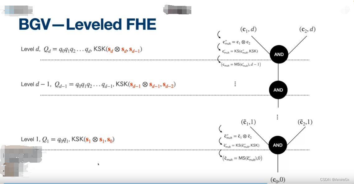
同态方案

方案算法：

• $\mathsf{F}\mathsf{H}\mathsf{E}.\mathsf{S}\mathsf{e}\mathsf{t}\mathsf{u}\mathsf{p}(1^{\lambda },1^L,b)$:

  1. 输入安全参数、级别数和用来确定用LWE还是RLWE的参数，设$\mu =\mu (\lambda ,L,b)=\theta (\log \lambda +\log L)$.
  2. 对于每个$j=L$(电路输入层) $\text{ to }0$(电路输出层):执行$param{s}_j\leftarrow \mathsf{E}.\mathsf{S}\mathsf{e}\mathsf{t}\mathsf{u}\mathsf{p}(1^{\lambda },1^{(j+1)\cdot \mu },b)$, 生成一个阶梯式的模数（从$q_L((L+1)\cdot \mu bits)$降低到$q_0(\mu bits)$
  3. 对于每个$j=L-1\text{ to }0$
     令$d_j=d_L$, ${\chi }_j={\chi }_L$。此外, 每一层的$d,\chi$参数需要与$L$层统一, 而维数$n$则没有这个要求.（这是由于在$q$变小时, 维数的减少不会影响方案的安全性, 毕竟当$q$下降时, 维数的减小不会让破解变得容易)

• F H E . K e y G e n ( { p a r a m s j } ) \mathsf{FHE.KeyGen}(\{params_j\}) FHE.KeyGen({ paramsj​}):

  1. 对于每个$j=L\text{ to }0$, 执行:
     执行${\mathbf{s}}_j\leftarrow \mathsf{E}.\mathsf{S}\mathsf{e}\mathsf{c}\mathsf{r}\mathsf{e}\mathsf{t}\mathsf{K}\mathsf{e}\mathsf{y}\mathsf{G}\mathsf{e}\mathsf{n}(params{s}_j)$和${\mathbf{A}}_j\leftarrow \mathsf{E}.\mathsf{P}\mathsf{u}\mathsf{b}\mathsf{l}\mathsf{i}\mathsf{c}\mathsf{K}\mathsf{e}\mathsf{y}\mathsf{G}\mathsf{e}\mathsf{n}(param{s}_j,{\mathbf{s}}_j)$
  2. 令${\mathbf{s}}_j^{\prime }\leftarrow {\mathbf{s}}_j\otimes {\mathbf{s}}_j$。
  3. 令${\mathbf{s}}_j^{\prime \prime }\leftarrow \mathsf{B}\mathsf{i}\mathsf{t}\mathsf{D}\mathsf{e}\mathsf{c}\mathsf{o}\mathsf{m}\mathsf{p}({\mathbf{s}}_j^{\prime },q_j)$.（以$\log q$位二进制展开）
  4. 令${\tau }_{{\mathbf{s}}_j^{\prime \prime }\to {\mathbf{s}}_{j-1}}\leftarrow \mathsf{S}\mathsf{w}\mathsf{i}\mathsf{t}\mathsf{c}\mathsf{h}\mathsf{K}\mathsf{e}\mathsf{y}\mathsf{G}\mathsf{e}\mathsf{n}({\mathbf{s}}_j^{\prime \prime },{\mathbf{s}}_{j-1})$ (当$j=L$时不执行该步骤)。
     实际上上述算法中, 我们就生成了每一层的公私钥, 并且做好了每一层的${\tau }_{{\mathbf{s}}_j^{\prime \prime }\to {\mathbf{s}}_{j-1}}$。

• F H E . E n c ( p a r a m s , p k , m ∈ { 0 , 1 } ) \mathsf{FHE.Enc}(params,pk,m\in\{0,1\}) FHE.Enc(params,pk,m∈{ 0,1}): 计算并输出$\mathsf{E}.\mathsf{E}\mathsf{n}\mathsf{c}({\mathbf{A}}_L,m)$.

• $\mathsf{F}\mathsf{H}\mathsf{E}.\mathsf{D}\mathsf{e}\mathsf{c}(params,sk,\mathbf{c})$: 根据密钥的层数选择${\mathbf{s}}_j$, 计算并输出$\mathsf{E}.\mathsf{D}\mathsf{e}\mathsf{c}({\mathbf{s}}_j,\mathbf{c})$.
  此处我们忽略了确定密文层数的参数来化简表示，原文写的可以使用一个指示参数来指定。

同态计算中要用到模数交换过程和密钥交换过程, 作者将其统一为一个$\mathsf{R}\mathsf{e}\mathsf{f}\mathsf{r}\mathsf{e}\mathsf{s}\mathsf{h}$过程：首先要根据计算密钥的格式, 将乘法(或加法)得到的结果进行$\mathsf{P}\mathsf{o}\mathsf{w}\mathsf{e}\mathsf{r}\mathsf{o}\mathsf{f}2$操作, 然后依次进行模数切换和密钥切换，即，把一个${\mathbf{s}}_j’={\mathbf{s}}_j\otimes {\mathbf{s}}_j$下得密文变为${\mathbf{s}}_{j-1}$下得密文.。

• $\mathsf{F}\mathsf{H}\mathsf{E}.\mathsf{R}\mathsf{e}\mathsf{f}\mathsf{r}\mathsf{e}\mathsf{s}\mathsf{h}(\mathbf{c},{\tau }_{{\mathbf{s}}_j^{\prime \prime }\to {\mathbf{s}}_{j-1},q_j,q_{j-1}})$:
  输入的是一个由${\mathbf{s}}_j^{\prime }$加密的密文、密钥交换辅助信息，当前层和下一层的模数。
  1. 扩张密文，使得密文与密钥的内积不变。计算${\mathbf{c}}_1\leftarrow \mathsf{P}\mathsf{o}\mathsf{w}\mathsf{e}\mathsf{r}\mathsf{o}\mathsf{f}2(\mathbf{c},q_j)$（这里能想到$<{\mathbf{c}}_1,{\mathbf{s}}_j^{\prime \prime }>=<\mathbf{c},{\mathbf{s}}_j^{\prime }>$ 从前面的二进制转换那里能总结出来）
  2. 模交换，计算${\mathbf{c}}_2\leftarrow \mathsf{S}\mathsf{c}\mathsf{a}\mathsf{l}\mathsf{e}({\mathbf{c}}_1,q_j,q_{j-1},2)$
  3. 密钥交换，计算并输出${\mathbf{c}}_3\leftarrow \mathsf{S}\mathsf{w}\mathsf{i}\mathsf{t}\mathsf{c}\mathsf{h}\mathsf{K}\mathsf{e}\mathsf{y}({\tau }_{{\mathbf{s}}_j’’\to {\mathbf{s}}_{j-1}},{\mathbf{c}}_2,q_{j-1})$

最后我们补充完同态借助$\mathsf{R}\mathsf{e}\mathsf{f}\mathsf{r}\mathsf{e}\mathsf{s}\mathsf{h}$完成的同态运算过程（输入的两个密文都是同一个密钥加密出来的）:

• $\mathsf{F}\mathsf{H}\mathsf{E}.\mathsf{A}\mathsf{d}\mathsf{d}(pk,{\mathbf{c}}_1,{\mathbf{c}}_2)$:
  首先计算${\mathbf{c}}_3={\mathbf{c}}_1+{\mathbf{c}}_2$, 再计算输出${\mathbf{c}}_4=\mathsf{F}\mathsf{H}\mathsf{E}.\mathsf{R}\mathsf{e}\mathsf{f}\mathsf{r}\mathsf{e}\mathsf{s}\mathsf{h}({\mathbf{c}}_3,q_j,q_{j-1})$。（有需要就调用刷新）
• $\mathsf{F}\mathsf{H}\mathsf{E}.\mathsf{M}\mathsf{u}\mathsf{l}\mathsf{t}(pk,{\mathbf{c}}_1,{\mathbf{c}}_2)$:
  首先计算${\mathbf{c}}_3$, 即由${\mathbf{c}}_1,{\mathbf{c}}_2$所表示的多项式函数相乘得到的多项式函数对应的密文, 再计算并输出${\mathbf{c}}_4=\mathsf{F}\mathsf{H}\mathsf{E}.\mathsf{R}\mathsf{e}\mathsf{f}\mathsf{r}\mathsf{e}\mathsf{s}\mathsf{h}({\mathbf{c}}_3,q_j,q_{j-1})$。

最后来看看整个方案的噪声增长：

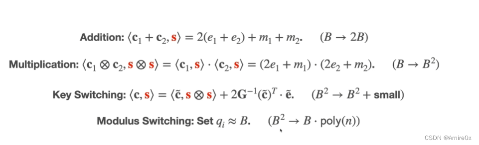
在密钥交换和模交换后都会诞生一部分小的噪声，如果在模交换的时候设置模数为$q$，那么乘法后的噪声就是$B^2/(B+small)\to B\cdot poly(n)$

参考

同态加密(3) BGV方案

全同态加密：BGV

同态加密（七）无自举的分级全同态加密 1 (Leveled)Fully Homomorphic Encryption without Bootstrapping

Brakerski Z, Gentry C, Vaikuntanathan V. (Leveled) fully homomorphic encryption without bootstrapping[J]. ACM Transactions on Computation Theory (TOCT), 2014, 6(3): 1-36.

全同态加密I：理论与基础