机器学习——分类问题(2020最新版)

直接使用梯度下降法去做逻辑回归，相当于完成底层实现。

直接调用sklearn的话，简单很多，具体实现无法学习到。

一、逻辑回归(Logistic Regression)

逻辑回归是用来处理分类问题的

Sigmoid/Logistic Function:

1、决策边界

case 1:

扫描二维码关注公众号，回复： 11562668 查看本文章

case 2:

case 3:

2、逻辑回归的代价函数

(1) 所以对于non-convex func来说，梯度下降法的代价函数并不适合这种问题求解，需要新的代价函数。

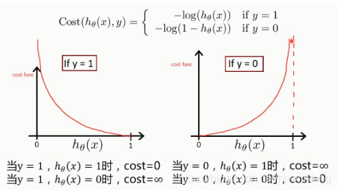
(2) 由上图可知，预测正确，cost的值越小(为0)，预测错误，cost的值越大(为无穷大)。

(3) 这个就是逻辑回归的代价函数的公式，在后面深度学习里面使用的交叉熵，也是这个公式。

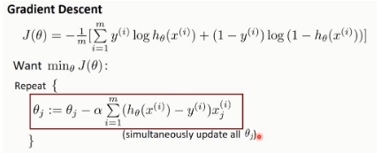
使用梯度下降法，下面是求导过程：

所以得到@j的每次更替的值用如下式子进行赋值：

3、多分类问题如何解决

逻辑回归一般是用来做这种二分类的问题的，那么对于多分类的情况，如何做？

可以做三个分类边界，如下图：

4、逻辑回归的正则化

——————————————————————————————————————————

在上面的介绍如何使用逻辑回归进行分类后，下面讲述如何去评价分类后的结果（评价指标）

——————————————————————————————————————————

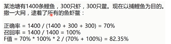
5、正确率(precision)/召回率(recall)/F1指标

举个例子，去理解正确率、召回率、F1-score：

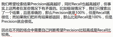
因此，综合考虑precision和recall才是可行的，所以使用F1-Score来评价：

使用最基本的梯度下降法来实现线性逻辑回归：

# -*- coding: utf-8 -*- #
"""
-------------------------------------------------------------------------------
  FileName:    sks_logistic_regression_method
  Author:      newlinfeng
  Date:        2020/7/28 0028  11:47
  Description: 使用sklearn实现分类问题中的逻辑回归
-------------------------------------------------------------------------------
"""
import matplotlib.pyplot as plt
import numpy as np
from sklearn.metrics import classification_report
from sklearn import preprocessing

# 数据是否需要标准化
scale = False

# 载入数据
data = np.genfromtxt(r"LR-testSet.csv", delimiter=",")
x_data = data[:, :-1]
y_data = data[:, -1]

#为了画这个散点图
def plot():
    x0 = []
    x1 = []
    y0 = []
    y1 = []
    #切分不同类型的数据
    for i in range(len(x_data)):
        if y_data[i] == 0:
            x0.append(x_data[i, 0])
            y0.append(x_data[i, 1])
        else:
            x1.append(x_data[i, 0])
            y1.append(x_data[i, 1])
    #画图
    scatter0 = plt.scatter(x0, y0, c='b', marker='o')
    scatter1 = plt.scatter(x1, y1, c='r', marker='x')
    #画图例
    plt.legend(handles=[scatter0, scatter1], labels=['label0', 'label1'], loc='best')



#数据处理,添加偏执项
x_data = data[:, :-1]
y_data = data[:, -1, np.newaxis]

#给样本添加偏执项
X_data = np.concatenate((np.ones((100, 1)), x_data), axis=1)

#逻辑回归的函数
def sigmoid(x):
    return 1.0/(1+np.exp(-x))

#逻辑回归的代价函数
def cost(xMat, yMat, ws):
    left = np.multiply(yMat, np.log(sigmoid(xMat*ws))) #multiply()是对于矩阵元素的位置进行相乘(矩阵的形状必须一模一样)
    right = np.multiply(1-yMat, np.log(1-sigmoid(xMat*ws)))
    return np.sum(left + right)/-(len(xMat))

#
def gradAscent(xArr, yArr):
    if scale == True:
        xArr = preprocessing.scale(xArr)
    xMat = np.mat(xArr)
    yMat = np.mat(yArr)

    lr = 0.001 #学习率
    epochs = 10000 #迭代周期
    costList = [] #保存cost的值
    #计算数据行列数
    #行代表数据个数，列代表权值个数
    m, n = np.shape(xMat)
    #初始化权值矩阵
    ws = np.mat(np.ones((n, 1)))

    for i in range(epochs+1):
        #xMat和weights矩阵相乘
        h = sigmoid(xMat*ws)
        #计算误差
        ws_grad = xMat.T*(h-yMat)/m
        ws = ws - lr*ws_grad

        if i%50 == 0:
            costList.append(cost(xMat, yMat, ws))
    return ws,costList

#训练模型，得到权重和cost值的变化
ws, costList = gradAscent(X_data, y_data)
print(ws)

#是否做参数标准化
if scale == False:
    #画图决策边界
    plot()
    #画那条线
    x_test = [[-4], [3]]
    y_test = (-ws[0] - x_test*ws[1])/ws[2]
    plt.plot(x_test, y_test, 'k')
    plt.show()

#画下loss值的变化
x = np.linspace(0, 10000, 201)
plt.plot(x, costList, c='r')
plt.title("Train")
plt.xlabel("Epochs")
plt.ylabel("Cost")
plt.show()

#预测
def predict(x_data, ws):
    if scale == True:
        x_data = preprocessing.scale(x_data)
    xMat = np.mat(x_data)
    ws = np.mat(ws)
    return [1 if x>=0.5 else 0 for x in sigmoid(xMat*ws)]

predictions = predict(X_data, ws)
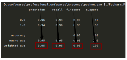
print(classification_report(y_data, predictions))

相应的评价指标值为：

使用sklearn来实现线性逻辑回归：

# -*- coding: utf-8 -*- #
"""
-------------------------------------------------------------------------------
  FileName:    skl_logistic_regression_method
  Author:      newlinfeng
  Date:        2020/7/28 0028  16:27
  Description: 使用sklearn实现逻辑回归
-------------------------------------------------------------------------------
"""
import matplotlib.pyplot as plt
import numpy as np
from sklearn.metrics import classification_report
from sklearn import preprocessing
from sklearn import linear_model
#数据是否需要标准化
scale = False

#载入数据
data = np.genfromtxt("LR-testSet.csv", delimiter=",")
x_data = data[:, :-1]
y_data = data[:, -1]

def plot():
    x0 = []
    x1 = []
    y0 = []
    y1 = []
    #切分不同类型的数据
    for i in range(len(x_data)):
        if y_data[i] == 0:
            x0.append(x_data[i, 0])
            y0.append(x_data[i, 1])
        else:
            x1.append(x_data[i, 0])
            y1.append(x_data[i, 1])
    #画图
    scatter0 = plt.scatter(x0, y0, c='b', marker='o')
    scatter1 = plt.scatter(x1, y1, c='r', marker='x')
    #画图例
    plt.legend(handles=[scatter0, scatter1], labels=['label0', 'label1'], loc='best')

plot()
plt.show()

logistic = linear_model.LogisticRegression()
logistic.fit(x_data, y_data)

if scale == False:
    #画决策边界
    plot()
    x_test = np.array([[-4], [3]])
    y_test = (-logistic.intercept_ - x_test*logistic.coef_[0][0]/logistic.coef_[0][1])
    plt.plot(x_test, y_test, 'k')
    plt.show()

predictions = logistic.predict(x_data)
print(classification_report(y_data, predictions))

结果比上面好一些：

6、非线性逻辑回归

使用梯度下降法实现非线性逻辑回归：

# -*- coding: utf-8 -*- #
"""
-------------------------------------------------------------------------------
  FileName:    gradAscent_logistic_regression
  Author:      newlinfeng
  Date:        2020/7/28 0028  17:07
  Description: 
-------------------------------------------------------------------------------
"""
import matplotlib.pyplot as plt
import numpy as np
from sklearn.metrics import classification_report
from sklearn import preprocessing
from sklearn.preprocessing import PolynomialFeatures
# 数据是否需要标准化
scale = False

# 载入数据
data = np.genfromtxt(r"LR-testSet2.txt", delimiter=",")
x_data = data[:, :-1]
y_data = data[:, -1, np.newaxis]

#为了画这个散点图
def plot():
    x0 = []
    x1 = []
    y0 = []
    y1 = []
    #切分不同类型的数据
    for i in range(len(x_data)):
        if y_data[i] == 0:
            x0.append(x_data[i, 0])
            y0.append(x_data[i, 1])
        else:
            x1.append(x_data[i, 0])
            y1.append(x_data[i, 1])
    #画图
    scatter0 = plt.scatter(x0, y0, c='b', marker='o')
    scatter1 = plt.scatter(x1, y1, c='r', marker='x')
    #画图例
    plt.legend(handles=[scatter0, scatter1], labels=['label0', 'label1'], loc='best')

plot()
plt.show()

#定义多项式回归，degree的值可以调节多项式的特征
poly_reg = PolynomialFeatures(degree=3)
#特征处理
x_poly = poly_reg.fit_transform(x_data)

#逻辑回归的函数
def sigmoid(x):
    return 1.0/(1+np.exp(-x))

#逻辑回归的代价函数
def cost(xMat, yMat, ws):
    left = np.multiply(yMat, np.log(sigmoid(xMat*ws))) #multiply()是对于矩阵元素的位置进行相乘(矩阵的形状必须一模一样)
    right = np.multiply(1-yMat, np.log(1-sigmoid(xMat*ws)))
    return np.sum(left + right)/-(len(xMat))

def gradAscent(xArr, yArr):
    if scale == True:
        xArr = preprocessing.scale(xArr)
    xMat = np.mat(xArr)
    yMat = np.mat(yArr)

    lr = 0.03 #学习率
    epochs = 50000 #迭代周期
    costList = [] #保存cost的值
    #计算数据行列数
    #行代表数据个数，列代表权值个数
    m, n = np.shape(xMat)
    #初始化权值矩阵
    ws = np.mat(np.ones((n, 1)))

    for i in range(epochs+1):
        #xMat和weights矩阵相乘
        h = sigmoid(xMat*ws)
        #计算误差
        ws_grad = xMat.T*(h-yMat)/m
        ws = ws - lr*ws_grad

        if i%50 == 0:
            costList.append(cost(xMat, yMat, ws))
    return ws,costList

#训练模型，得到权重和cost值的变化
ws, costList = gradAscent(x_poly, y_data)
print(ws)

#获取数据值所在的范围
x_min, x_max = x_data[:, 0].min() - 1, x_data[:, 0].max() + 1
y_min, y_max = x_data[:, 1].min() - 1, x_data[:, 1].max() + 1

#生成网格矩阵
xx, yy = np.meshgrid(np.arange(x_min, x_max, 0.02), np.arange(y_min, y_max, 0.02))

#ravel与flatten类似，多为数组转一维，flatten不会改变原始数据，ravel会改变
z = sigmoid(poly_reg.fit_transform(np.c_[xx.ravel(), yy.ravel()]).dot(np.array(ws)))
for i in range(len(z)):
    if z[i] > 0.5:
        z[i] = 1
    else:
        z[i] = 0
z = z.reshape(xx.shape)

#等高线图
cs = plt.contourf(xx, yy, z)
plot()
plt.show()

#预测
def predict(x_data, ws):
    xMat = np.mat(x_data)
    ws = np.mat(ws)
    return [1 if x >= 0.5 else 0 for x in sigmoid(xMat*ws)]

predictions = predict(x_poly, ws)
print(classification_report(y_data, predictions))

使用sklearn实现非线性逻辑回归：

# -*- coding: utf-8 -*- #
"""
-------------------------------------------------------------------------------
  FileName:    skl_logistic_regression_method
  Author:      newlinfeng
  Date:        2020/7/28 0028  17:45
  Description: 使用sklearn实现非线性逻辑回归
-------------------------------------------------------------------------------
"""
import numpy as np
import matplotlib.pyplot as plt
from sklearn import linear_model
from sklearn.datasets import make_gaussian_quantiles
from sklearn.preprocessing import PolynomialFeatures

#生成一个二维正态分布，生成的数据按照分位数分成两类，500个样本，2个样本特征
#可以生成两类或多类数据
x_data, y_data = make_gaussian_quantiles(n_samples=500, n_features=2, n_classes=2)

plt.scatter(x_data[:, 0], x_data[:, 1], c=y_data)
plt.show()

logistic = linear_model.LogisticRegression()
logistic.fit(x_data, y_data)

#获取数据值所在的范围
x_min, x_max = x_data[:, 0].min() - 1, x_data[:, 0].max() + 1
y_min, y_max = x_data[:, 1].min() - 1, x_data[:, 1].max() + 1

#生成网格矩阵
xx, yy = np.meshgrid(np.arange(x_min, x_max, 0.02), np.arange(y_min, y_max, 0.02))

#ravel与flatten类似，多维数据转一维。flatten不会改变原始数据，ravel会改变原始数据
z = logistic.predict(np.c_[xx.ravel(), yy.ravel()])
z = z.reshape(xx.shape)
#等高线图
cs = plt.contourf(xx, yy, z)
#样本散点图
plt.scatter(x_data[:, 0], x_data[:, 1], c=y_data)
plt.show()

print('score:', logistic.score(x_data, y_data))

#定义多项式回归，degree的值可以调节多项式的特征
poly_reg = PolynomialFeatures(degree=5)
#特征处理
x_poly = poly_reg.fit_transform(x_data)
#定义逻辑回归模型
logistic = linear_model.LogisticRegression()
#训练模型
logistic.fit(x_poly, y_data)

#获取数据值所在的范围
x_min, x_max = x_data[:, 0].min()-1, x_data[:, 0].max()+1
y_min, y_max = x_data[:, 1].min()-1, x_data[:, 1].max()+1

#生成网格矩阵
xx, yy = np.meshgrid(np.arange(x_min, x_max, 0.02), np.arange(y_min, y_max, 0.02))

#ravel和flatten类似,多维数据转一维。flatten不会改变原始数据,ravel会改变原始数据
z = logistic.predict(poly_reg.fit_transform(np.c_[xx.ravel(), yy.ravel()]))
z = z.reshape(xx.shape)
#等高线图
cs = plt.contourf(xx, yy, z)
#样本散点图
plt.scatter(x_data[:, 0], x_data[:, 1], c=y_data)
plt.show()

print('score:', logistic.score(x_poly, y_data))

2020-07-31更新