1、深度学习三次热潮


2、深度学习爆发的三要素
大数据、计算能力、算法
3、深度学习三巨头(三个代表人物)


此外,还有一个人也是很著名的,华裔科学家吴恩达:

他们之间的关系网:

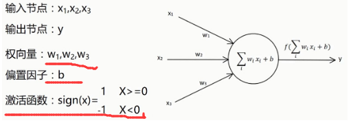
4、单层感知器
4.1 人体神经网络

人工设计的神经元:
例如:

另外一种神经元结构:

4.2 感知器的学习规则

例如:

学习率的取值:
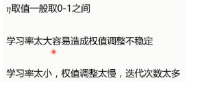
不同的学习率随着迭代次数的变化,loss值的变化:

模型收敛的条件(loss达到何值时收敛?):

4.3 单层感知器程序

单层感知器程序:
# -*- coding: utf-8 -*- #
"""
-------------------------------------------------------------------------------
  FileName:    sig_layer_perception
  Author:      newlinfeng
  Date:        2020/7/29 0029  22:05
  Description: 关于单层感知器的题目,每次的运行结果都是不一样的
-------------------------------------------------------------------------------
"""
import numpy as np
import matplotlib.pyplot as plt

#输入数据
X = np.array([[1, 3, 3],
              [1, 4, 3],
              [1, 1, 1],
              [1, 0, 2]])
#标签
Y = np.array([[1],
              [1],
              [-1],
              [-1]])

#权值初始化,3行1列,数值范围-1到1
W = (np.random.random([3, 1])-0.5)*2
print(W)

#学习率的设置
lr = 0.11
#神经网络输出
O = 0

#用来更新权值矩阵的函数
def update():
    global X, Y, W, lr
    O = np.sign(np.dot(X, W)) #shape:(3, 1)
    W_C = lr*(X.T.dot(Y-O))/int(X.shape[0])
    W = W + W_C

for i in range(100):
    update()#更新权值
    print(W)#打印当前权值
    print(i)#打印当前迭代次数
    O = np.sign(np.dot(X, W))#计算当前输出
    #all() O、Y矩阵(4*1)完全表示完全相等时
    if(O == Y).all(): #如果实际输出等于期望输出,模型收敛,循环结束
        print("Finished")
        print('epoch:', i)#打印当前迭代次数
        break

#正样本
x1 = [3, 4]
y1 = [3, 3]
#负样本
x2 = [1, 0]
y2 = [1, 2]

#计算分界线的斜率以及截距,依据w0+x*w1+y*w2 = 0求出的斜率和截距
k = -W[1]/W[2]
d = -W[0]/W[2]
print('k=', k)
print('d=', d)

xdata = (0, 5)

plt.figure()
plt.plot(xdata, xdata*k+d, 'r')
plt.scatter(x1, y1, c='b')
plt.scatter(x2, y2, c='y')
plt.show()
4.4 单层感知器-异或问题
异或:如果a、b两个值不相同,则异或结果为1。如果a、b两个值相同,异或结果为0。
或:是有真就是真;
同或:同真,不同假;
异或:同假,不同真;
单层感知器-异或问题:对于测试点,无法使用直线来分割,例如如下程序的结果(非线性问题),即使用单层感知器无法解决这个问题。
# -*- coding: utf-8 -*- #
"""
-------------------------------------------------------------------------------
  FileName:    sig_layer_perception_异或
  Author:      newlinfeng
  Date:        2020/7/31 0031  14:32
  Description: 单层感知器的异或问题(无法解决,但是使用线性神经网络可以解决)
-------------------------------------------------------------------------------
"""
import numpy as np
import matplotlib.pyplot as plt

# 输入数据
X = np.array([[1, 0, 0],
              [1, 0, 1],
              [1, 1, 0],
              [1, 1, 1]])

# 标签
Y = np.array([[-1],
              [1],
              [1],
              [-1]])

# 权值初始化
W = (np.random.random([3, 1]) - 0.1) * 2

print(W)
# 学习率的设置
lr = 0.11
# 神经网络的输出
O = 0


def update():
    global X, Y, W, lr
    O = np.sign(np.dot(X, W))  # shape:(3, 1)
    W_C = lr * (X.T.dot(Y - O)) / int(X.shape[0])
    W = W + W_C


for i in range(100):
    update()  # 更新权值
    print(i)  # 打印迭代次数
    O = np.sign(np.dot(X, W))  # 计算当前输出
    if (O == Y).all():  # 如果实际输出等于期望输出,模型收敛,循环结束
        print("Finished")
        print('epoch:', i)
        break

# 正样本
x1 = [0, 1]
y1 = [1, 0]
# 负样本
x2 = [0, 1]
y2 = [0, 1]

# 计算分界线的斜率以及截距
k = -W[1] / W[2]
b = -W[0] / W[2]

print('k=', k)
print('b=', b)

xdata = (-2, 3)
plt.figure()
plt.plot(xdata, xdata * k + b, 'r')
plt.scatter(x1, y1, c='b')
plt.scatter(x2, y2, c='y')
plt.show()

(1) 具体使用什么方法来解决非线性的问题,后面会给出解决方案。
5、线性神经网络、Delta学习规则
5.1 线性神经网络(linear neural network)
线性神经网络在结构上与感知器非常相似,只是激活函数不同。在模型训练时把原来的sign函数改成了purelin函数:y=x。
使用purelin作为激活函数的程序:
# -*- coding: utf-8 -*- #
"""
-------------------------------------------------------------------------------
  FileName:    linear_neural_network
  Author:      newlinfeng
  Date:        2020/7/31 0031  14:56
  Description: 线性神经网络-purelin函数
-------------------------------------------------------------------------------
"""
import numpy as np
import matplotlib.pyplot as plt

#输入数据
X = np.array([[1, 3, 3],
              [1, 4, 3],
              [1, 1, 1],
              [1, 0, 2]])

#标签
Y = np.array([[1],
              [1],
              [-1],
              [-1]])

#权值初始化,3行1列,取值范围-1到1
W = (np.random.random([3, 1])-0.5)*2

print(W)
#学习率设置
lr = 0.11
#神经网络输出
O = 0

def update():
    global X, Y, W, lr
    O = np.dot(X, W) #单层感知器使用的激活函数是np.sign(np.dot(X, W))
    W_C = lr*(X.T.dot(Y-O))/int(X.shape[0])
    W += W_C

for _ in range(100):
    update()
    # 正样本
    x1 = [3, 4]
    y1 = [3, 3]
    # 负样本
    x2 = [1, 0]
    y2 = [1, 2]

    # 计算分界线的斜率以及截距,依据w0+x*w1+y*w2 = 0求出的斜率和截距
    k = -W[1] / W[2]
    d = -W[0] / W[2]
    print('k=', k)
    print('d=', d)

    xdata = (0, 5)

    plt.figure()
    plt.plot(xdata, xdata * k + d, 'r')
    plt.scatter(x1, y1, c='b')
    plt.scatter(x2, y2, c='y')
    plt.show()

还有很多的激活函数类别,比如:

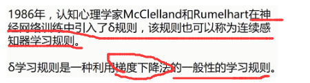
5.2 Delta函数(调整权值W的一种方法)
(1) 而之前使用的感知器的学习规则(调整w)是很简单的,如下图:
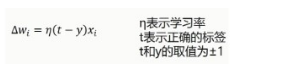
Delta函数学习规则:

关于梯度下降法-一维情况:

关于梯度下降法-二维情况:

梯度下降法的问题:

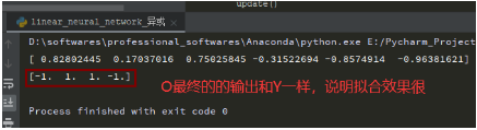
5.3 解决异或问题(使用线性神经网络来做)

我这里使用第二种方案:引入非线性的输入,再加一些输入项,再做神经网络——从而解决异或问题。
# -*- coding: utf-8 -*- #
"""
-------------------------------------------------------------------------------
  FileName:    linear_neural_network_异或
  Author:      newlinfeng
  Date:        2020/7/31 0031  17:35
  Description: 使用线性神经网络+第二种方案解决异或问题
-------------------------------------------------------------------------------
"""
import numpy as np
import matplotlib.pyplot as plt

# 输入数据
X = np.array([[1, 0, 0, 0, 0, 0],
              [1, 0, 1, 0, 0, 1],
              [1, 1, 0, 1, 0, 0],
              [1, 1, 1, 1, 1, 1]])
# 标签
Y = np.array([-1, 1, 1, -1])

# 权值初始化,6行1列,数值范围-1到1
W = (np.random.random(6) - 0.5) * 2
print(W)

# 学习率的设置
lr = 0.11
# 计算迭代次数
n = 0
# 神经网络输出
O = 0


# 用来更新权值矩阵的函数
def update():
    global X, Y, W, lr, n
    n += 1
    O = np.dot(X, W.T)
    W_C = lr * (X.T.dot(Y - O.T)) / int(X.shape[0])
    W = W + W_C


for _ in range(10000):
    update()  # 更新权值

# 正样本
x1 = [0, 1]
y1 = [1, 0]
# 负样本
x2 = [0, 1]
y2 = [0, 1]


def calculate(x, root):
    a = W[5]
    b = W[2] + x * W[4]
    c = W[0] + x * W[1] + x * x * W[3]
    if root == 1:
        return (-b + np.sqrt(b * b - 4 * a * c)) / (2 * a)
    if root == 2:
        return (-b - np.sqrt(b * b - 4 * a * c)) / (2 * a)


xdata = np.linspace(-1, 2)

plt.figure()
plt.plot(xdata, calculate(xdata, 1), 'r')
plt.plot(xdata, calculate(xdata, 2), 'r')
plt.plot(x1, y1, 'bo')
plt.plot(x2, y2, 'yo')
plt.show()

O = np.dot(X, W.T)
print(O)
6、BP神经网络(Back Propagation Neural Network)反向传播
6.1 BP神经网络的由来

6.2 网络结构


(1) 关于BP算法的推到过程,可以后面的推导过程
例如:

6.3 几种常用的激活函数
<1> Sigmoid函数(就是之前的逻辑回归的那个 函数):

<2> Tanh函数、Softsign函数

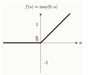
<3> ReLU函数(用的最多的激活函数)
6.4 BP神经网络推导(Back Propagation Neural Network)
空!
6.5 BP神经网络应用(解决异或问题)
# -*- coding: utf-8 -*- #
"""
-------------------------------------------------------------------------------
  FileName:    BP_neural_network_异或
  Author:      newlinfeng
  Date:        2020/8/1 0001  7:58
  Description: 使用BP(反向传播)神经网络解决异或问题
-------------------------------------------------------------------------------
"""
# 输入数据
import numpy as np

X = np.array([[1, 0, 0],
              [1, 0, 1],
              [1, 1, 0],
              [1, 1, 1]])
# 标签
Y = np.array([[0, 1, 1, 0]])

# 权值初始化,二层,数值范围-1到1
V = np.random.random((3, 4)) * 2 - 1
W = np.random.random((4, 1)) * 2 - 1
print(V)
print(W)

# 学习率的设置
lr = 0.11


# sigmoid函数的定义
def sigmoid(x):
    return 1 / (1 + np.exp(-x))


# sigmoid函数的导数
def dsigmoid(x):
    return x*(1 - x)


# 定义一个更新权值的函数
def update():
    global X, Y, W, V, lr
    # 隐藏层的输出(4, 4)
    L1 = sigmoid(np.dot(X, V))
    # 输出层的输出(4, 1)
    L2 = sigmoid(np.dot(L1, W))

    L2_delta = (Y.T - L2) * dsigmoid(L2)
    L1_delta = L2_delta.dot(W.T) * dsigmoid(L1)

    W_C = lr * L1.T.dot(L2_delta)
    V_C = lr * X.T.dot(L1_delta)

    W = W + W_C
    V = V + V_C


for i in range(20000):
    update()
    if i%50 == 0:
        L1 = sigmoid(np.dot(X, V))
        L2 = sigmoid(np.dot(L1, W))
        print('Error:', np.mean(np.abs(Y.T-L2)))
L1 = sigmoid(np.dot(X, V))
L2 = sigmoid(np.dot(L1, W))
print(L2)
6.6 BP神经网络的一篇论文
Understanding the difficulty of training deep feedforward neural networks
6.7 Google神经网络演示平台
网址:http://playground.tensorflow.org/ ,可以自己去玩一玩

2020-08-10 更新