Pytorch フレームワーク学習パス (5: autograd とロジスティック回帰)
記事ディレクトリ
オートグラード
torch.autograd.backward メソッドの導出
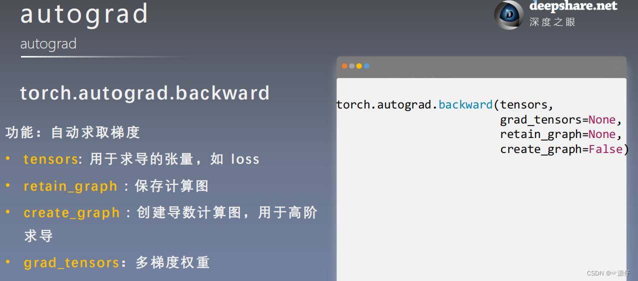
| 0、後方() |
コードは以下のように表示されます:
import torch
torch.manual_seed(10)


# ====================================== retain_graph ==============================================
flag = True
# flag = False
if flag:
    w = torch.tensor([1.], requires_grad=True)
    x = torch.tensor([2.], requires_grad=True)

    a = torch.add(w, x)
    b = torch.add(w, 1)
    y = torch.mul(a, b)

    y.backward()  # 反向传播
    print(w.grad)
    # y.backward()
外:
tensor([5.])
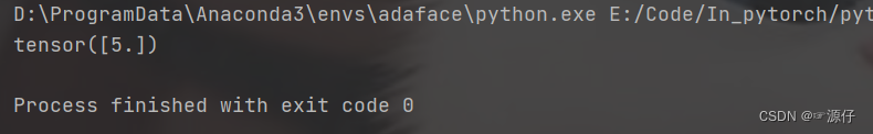
バックプロパゲーションを 2 回実行するとどうなるでしょうか?
import torch
torch.manual_seed(10)


# ====================================== retain_graph ==============================================
flag = True
# flag = False
if flag:
    w = torch.tensor([1.], requires_grad=True)
    x = torch.tensor([2.], requires_grad=True)

    a = torch.add(w, x)
    b = torch.add(w, 1)
    y = torch.mul(a, b)

    y.backward()  # 反向传播
    print(w.grad)
    y.backward()
外:
![テンソル([5.])](https://img-blog.csdnimg.cn/56063d706eee4a91a98a8160de085971.png)
- ほら、2回目のバックプロパゲーションをコンピュータで計算しようとしているというエラーが報告されましたが、保存された計算グラフは公開されています。
- 解決策: 初めてバックプロパゲーションを計算するときに、retain_graph=True を追加します。具体的なコードは次のとおりです。
# ====================================== retain_graph ==============================================
flag = True
# flag = False
if flag:
    w = torch.tensor([1.], requires_grad=True)
    x = torch.tensor([2.], requires_grad=True)

    a = torch.add(w, x)
    b = torch.add(w, 1)
    y = torch.mul(a, b)

    y.backward(retain_graph=True)  # retain_graph=True
    print(w.grad)
    y.backward()
外:
| 1、torch.autograd.backward |
今まで言ってきましたが
backward、これからも言うつもりはありませんかtorch.autograd.backward?実際にbackward、torch.autograd.backward以下のソースコードを見てみましょうbackward。
    def backward(self, gradient=None, retain_graph=None, create_graph=False, inputs=None):
        r"""Computes the gradient of current tensor w.r.t. graph leaves.

        The graph is differentiated using the chain rule. If the tensor is
        non-scalar (i.e. its data has more than one element) and requires
        gradient, the function additionally requires specifying ``gradient``.
        It should be a tensor of matching type and location, that contains
        the gradient of the differentiated function w.r.t. ``self``.

        This function accumulates gradients in the leaves - you might need to zero
        ``.grad`` attributes or set them to ``None`` before calling it.
        See :ref:`Default gradient layouts<default-grad-layouts>`
        for details on the memory layout of accumulated gradients.

        .. note::

            If you run any forward ops, create ``gradient``, and/or call ``backward``
            in a user-specified CUDA stream context, see
            :ref:`Stream semantics of backward passes<bwd-cuda-stream-semantics>`.

        Args:
            gradient (Tensor or None): Gradient w.r.t. the
                tensor. If it is a tensor, it will be automatically converted
                to a Tensor that does not require grad unless ``create_graph`` is True.
                None values can be specified for scalar Tensors or ones that
                don't require grad. If a None value would be acceptable then
                this argument is optional.
            retain_graph (bool, optional): If ``False``, the graph used to compute
                the grads will be freed. Note that in nearly all cases setting
                this option to True is not needed and often can be worked around
                in a much more efficient way. Defaults to the value of
                ``create_graph``.
            create_graph (bool, optional): If ``True``, graph of the derivative will
                be constructed, allowing to compute higher order derivative
                products. Defaults to ``False``.
            inputs (sequence of Tensor): Inputs w.r.t. which the gradient will be
                accumulated into ``.grad``. All other Tensors will be ignored. If not
                provided, the gradient is accumulated into all the leaf Tensors that were
                used to compute the attr::tensors. All the provided inputs must be leaf
                Tensors.
        """
        if has_torch_function_unary(self):
            return handle_torch_function(
                Tensor.backward,
                (self,),
                self,
                gradient=gradient,
                retain_graph=retain_graph,
                create_graph=create_graph,
                inputs=inputs)
        torch.autograd.backward(self, gradient, retain_graph, create_graph, inputs=inputs)
| 2、grad_tensors: マルチ勾配の重み |
# ====================================== grad_tensors ==============================================
flag = True
# flag = False
if flag:
    w = torch.tensor([1.], requires_grad=True)
    x = torch.tensor([2.], requires_grad=True)

    a = torch.add(w, x)     # retain_grad()
    b = torch.add(w, 1)

    y0 = torch.mul(a, b)    # y0 = (x+w) * (w+1)
    y1 = torch.add(a, b)    # y1 = (x+w) + (w+1)    dy1/dw = 2

    loss = torch.cat([y0, y1], dim=0)       # [y0, y1]
    print("Loss = {}".format(loss))
    grad_tensors = torch.tensor([1., 2.])

	# gradient=grad_tensors:多个梯度之间权重的设置。
    loss.backward(gradient=grad_tensors)    # gradient 传入 torch.autograd.backward()中的grad_tensors

    print("w.grad = {}".format(w.grad))
外:
Loss = tensor([6., 5.], grad_fn=<CatBackward>)
w.grad = tensor([9.])
大家可能这里有点懵,9是怎么来的?
loss式で表すと
、 loss = [ ( x + w ) × ( w + 1 ) , ( x + w ) + ( w + 1 ) ] loss = [(x+w)\times(w+1) , ( x +w)+(w+1)]ロス_ _ _=[ ( x+w)×( w+1 ) 、( ×+w)+( w+1 ) ] 、 x = 2 x = 2に入れる場合バツ=2およびw = 1 w=1w=1の場合、loss = tensor ( [ 6. , 5. ] loss = tensor([6., 5.]ロス_ _ _=テンソル( [ 6 . , _ _ _ _ _5.】loss勾配の計算: (以下で理解できますgradient=grad_tensors: 複数の勾配間の重みの設定)
∂ ( loss ) ∂ ( w ) = [ ( w + 1 ) + ( x + w ) , 2 ] \frac{\partial( loss)} {\partial(w)}=[(w+1)+(x+w) , 2]∂ ( w )∂ (ロス) _ _ _=[ ( w+1 )+( ×+w ) 、2 ] ,
{ ∣ ( w + 1 ) + ( x + w ) 2 ∣ × ∣ 1 2 ∣ } w = 1 , x = 2 = 9 \begin{Bmatrix} \begin{vmatrix} (w+1)+( x+w) & 2 \\ \end{vmatrix} \times \begin{vmatrix} 1\\ 2 \\ \end{vmatrix} \end{Bmatrix}_{w=1,x=2}= 9{ ∣∣( w+1 )+( ×+w )2∣∣×∣∣∣∣12∣∣∣∣}w = 1 、x = 2=9
torch.autograd.grad メソッドの導出
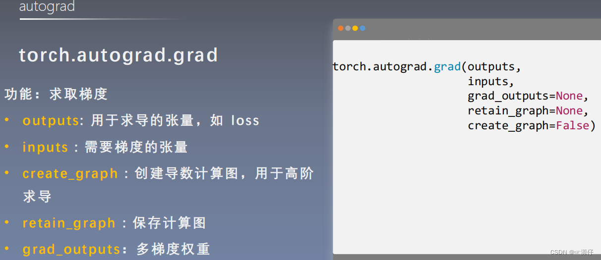
# ====================================== autograd.gard ==============================================
flag = True
# flag = False
if flag:

    x = torch.tensor([3.], requires_grad=True)
    y = torch.pow(x, 2)     # y = x**2

    grad_1 = torch.autograd.grad(y, x, create_graph=True)   # grad_1 = dy/dx = 2x = 2 * 3 = 6
    print("一次求导结果: {}".format(grad_1))

    grad_2 = torch.autograd.grad(grad_1[0], x)              # grad_2 = d(dy/dx)/dx = d(2x)/dx = 2
    print("二次求导结果: {}".format(grad_2))
外:
一次求导结果: (tensor([6.], grad_fn=<MulBackward0>),)
二次求导结果: (tensor([2.]),)
autograd のヒント (強調)
1. グラデーションが自動的にクリアされない
# ====================================== tips: 1 ==============================================
flag = True
# flag = False
if flag:

    w = torch.tensor([1.], requires_grad=True)
    x = torch.tensor([2.], requires_grad=True)

    for i in range(4):
        a = torch.add(w, x)
        b = torch.add(w, 1)
        y = torch.mul(a, b)

        y.backward()
        print(w.grad)

        # w.grad.zero_()
外:
tensor([5.])
tensor([10.])
tensor([15.])
tensor([20.])
pytorch上記の結果から、勾配が計算された後、勾配は自動的にクリアされないことがわかります0。累加计算そのため、正しい勾配結果を取得できません。したがって、手動でクリアする必要があり0ます。グラデーションをクリアします Clear to 0。
# ====================================== tips: 1 ==============================================
flag = True
# flag = False
if flag:

    w = torch.tensor([1.], requires_grad=True)
    x = torch.tensor([2.], requires_grad=True)

    for i in range(4):
        a = torch.add(w, x)
        b = torch.add(w, 1)
        y = torch.mul(a, b)

        y.backward()
        print(w.grad)

		# _符号指的是inplace操作.
        w.grad.zero_()
外:
tensor([5.])
tensor([5.])
tensor([5.])
tensor([5.])
リーフ ノードに依存するノード (requires_grad のデフォルトは True)
まずケースを見てみましょう: (バックプロパゲーションの前のwww 1)を追加します
flag = True
# flag = False
if flag:

    w = torch.tensor([1.], requires_grad=True)
    x = torch.tensor([2.], requires_grad=True)

    a = torch.add(w, x)
    b = torch.add(w, 1)
    y = torch.mul(a, b)

    w.add_(1)
    """
    autograd小贴士:
        梯度不自动清零
        依赖于叶子结点的结点,requires_grad默认为True
        叶子结点不可执行in-place
    """
    y.backward()

报错说:需要求导的叶变量执行了in-place操作。
什么叫in-place操作?看下面一段代码就能懂了.
# ====================================== tips: 3 ==============================================
flag = True
# flag = False
if flag:

    a = torch.ones((1, ))
    print("a 的地址                      : {}".format(id(a), a))

    # a = a + b这种形式会改变储存地址
    a = a + torch.ones((1, ))
    print("a + torch.ones((1, ))后的地址 : {} a = {}".format(id(a), a))

	# a += b这种形式会不改变储存地址
    a += torch.ones((1, ))
    print("a += torch.ones((1, ))后的地址: {} a = {}".format(id(a), a))
外:
a 的地址                      : 2168491070160
a + torch.ones((1, ))后的地址 : 2168584372088 a = tensor([2.])
a += torch.ones((1, ))后的地址: 2168584372088 a = tensor([3.])
那这种in-place操作(又叫原位操作)为啥在pytorch中要避免使用呢!
例:旅行中、旅行用品をギフトボックスに入れていたの
10号ですが、途中で誰かがスーツケースの商品を交換してしまった場合、その10号ブランドを利用してボックス内の商品を受け取る場合10号、その時にもらえるものはそのまま残りますか?同じですか? 計算図でも同じです. バックプロパゲーションのプロセスでは、初期w値を使用する必要があります。つまり、元のアドレスを使用して取得する必要があります。演算を使用すると、in-placeアドレスは変更されませんが、このアドレスに対応する値は元のw値ではなくなりました。
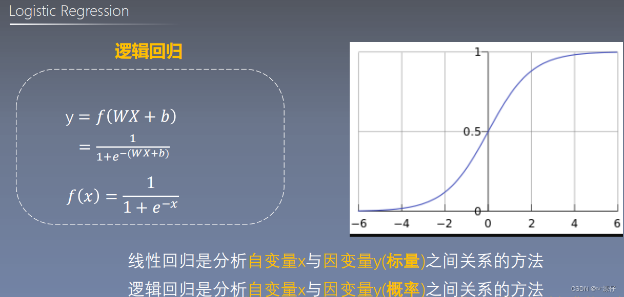
ロジスティック回帰
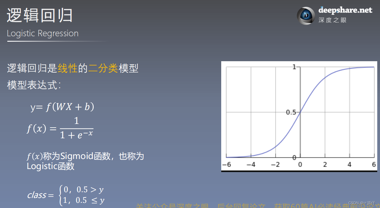
実際、
$WX + b$これも使用できます。当時は二分类同様でしたが、ニューロン(非線形)である確率分布に基づいており、分類効果は線形分類よりも優れていました。$WX + b > 0$$Sigmiod > 0.5$$WX + b < 0$$0 < Sigmiod < 0.5$Sigmiod1非线性作用函数
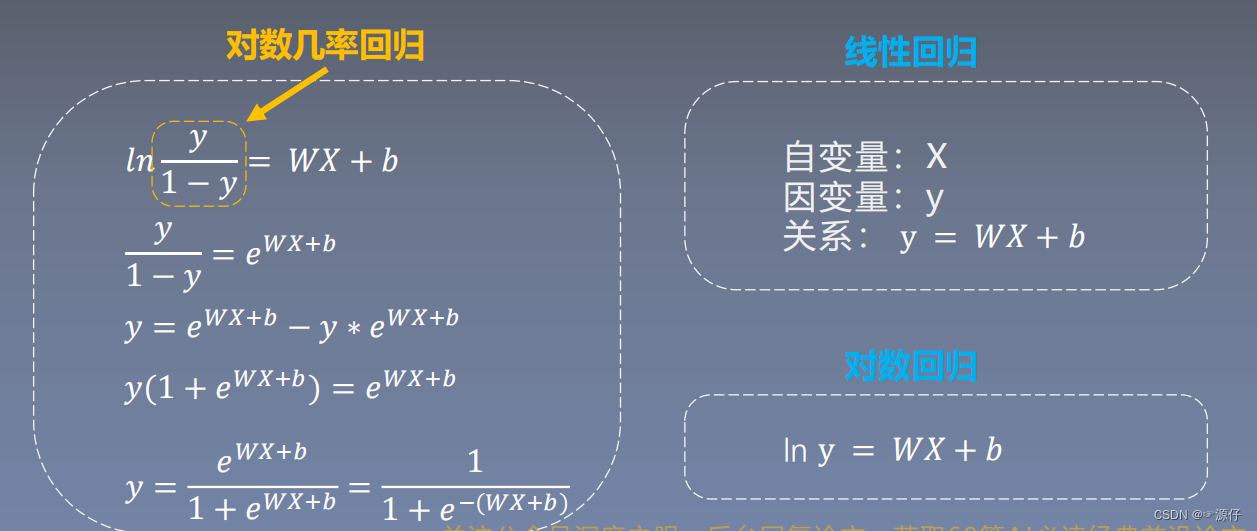
由上图可知,对数几率回归就等于逻辑回归,二者之间可通过转换得到。
| 線形バイナリ分類コードの例は次のとおりです。 |
線形バイナリ分類コードの例は次のとおりです。
import torch
import torch.nn as nn
import matplotlib.pyplot as plt
import numpy as np
torch.manual_seed(10)
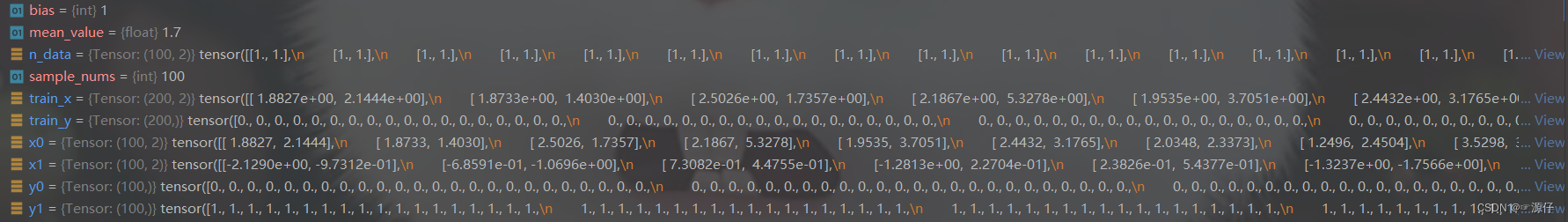
# ============================ step 1/5 生成数据 ============================
sample_nums = 100
mean_value = 1.7
bias = 1
n_data = torch.ones(sample_nums, 2)
# 生成均值为1.7,标准差为1的正态分布
x0 = torch.normal(mean_value * n_data, 1) + bias # 类别0 数据 shape=(100, 2)
y0 = torch.zeros(sample_nums) # 类别0 标签 shape=(100)
x1 = torch.normal(-mean_value * n_data, 1) + bias # 类别1 数据 shape=(100, 2)
y1 = torch.ones(sample_nums) # 类别1 标签 shape=(100)
train_x = torch.cat((x0, x1), 0)
train_y = torch.cat((y0, y1), 0)
# ============================ step 2/5 选择模型 ============================
class LR(nn.Module):
def __init__(self):
super(LR, self).__init__()
self.features = nn.Linear(2, 1)
self.sigmoid = nn.Sigmoid()
def forward(self, x):
x = self.features(x)
x = self.sigmoid(x)
return x
lr_net = LR() # 实例化逻辑回归模型
# ============================ step 3/5 选择损失函数 ============================
loss_fn = nn.BCELoss()
# ============================ step 4/5 选择优化器 ============================
lr = 0.01 # 学习率
optimizer = torch.optim.SGD(lr_net.parameters(), lr=lr, momentum=0.9)
# ============================ step 5/5 模型训练 ============================
for iteration in range(1000):
# 前向传播
y_pred = lr_net(train_x)
# 计算 loss
loss = loss_fn(y_pred.squeeze(), train_y)
# 反向传播
loss.backward()
# 更新参数
optimizer.step()
# 清空梯度
optimizer.zero_grad()
# 绘图
if iteration % 20 == 0:
mask = y_pred.ge(0.5).float().squeeze() # 以0.5为阈值进行分类
correct = (mask == train_y).sum() # 计算正确预测的样本个数
acc = correct.item() / train_y.size(0) # 计算分类准确率
plt.scatter(x0.data.numpy()[:, 0], x0.data.numpy()[:, 1], c='r', label='class 0')
plt.scatter(x1.data.numpy()[:, 0], x1.data.numpy()[:, 1], c='b', label='class 1')
w0, w1 = lr_net.features.weight[0]
w0, w1 = float(w0.item()), float(w1.item())
plot_b = float(lr_net.features.bias[0].item())
plot_x = np.arange(-6, 6, 0.1)
plot_y = (-w0 * plot_x - plot_b) / w1
plt.xlim(-5, 7)
plt.ylim(-7, 7)
plt.plot(plot_x, plot_y)
plt.text(-5, 5, 'Loss=%.4f' % loss.data.numpy(), fontdict={
'size': 20, 'color': 'red'})
plt.title("Iteration: {}\nw0:{:.2f} w1:{:.2f} b: {:.2f} accuracy:{:.2%}".format(iteration, w0, w1, plot_b, acc))
plt.legend()
plt.show()
plt.pause(0.5)
if acc > 0.99:
break
这时初学者可能对自定义的数据有些模糊,啥样的呢!如下图所示,这就不迷糊了(通透)。
训练过程展示: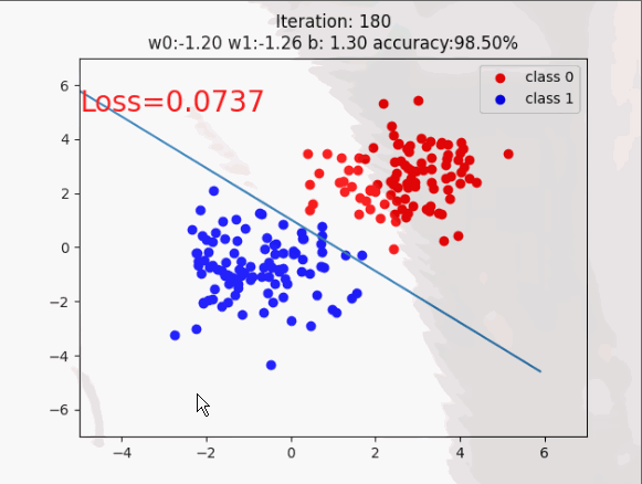
| 機械学習への 5 つのステップ |

上記のコードも機械学習の 5 つのステップに従っています。