목표 및 배경
목표: 거시 경제 주기 및 신용 카드 연체율의 선행 지표를 설정합니다.
데이터: 1990년부터 2008년까지 미국의 월간 거시 경제 데이터: 총 228개의 관측치, pce: 개인
소비 지출, 부채: 미결제 개인 소비 대출, 상환 비율: 채무 불이행 비율.
솔루션 및 절차
- 부채와 log(pce)의 산점도 만들기: 둘 사이에 강력한 선형 관계가 있습니다.
- 선형 회귀 모델을 설정하고 잔차를 구합니다. (경제적 설명)
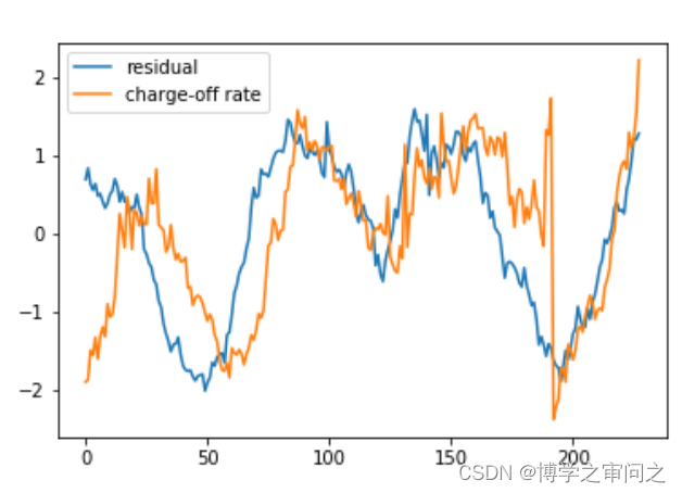
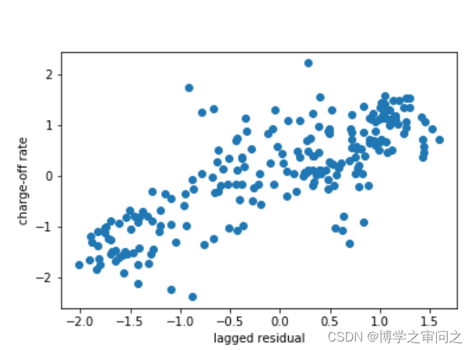
- 다음과 같이 기본 비율 및 잔차의 시퀀스 플롯과 지연된 잔차의 산점도를 그립니다.
- 기본 비율 대 히스테리시스 잔차를 선형 선형 모델로 추가로 모델링하거나
기본 비율 대 부채 및 로그(pce)를 히스테리시스로 직접 모델링할 수 있습니다.
pd
경로로 팬더 가져오기 = 'data/macro_econ_data.xls'
데이터 = pd.read_excel(경로)
부채 = data['회전 신용'].values[:,np.newaxis]
pce = data['명목 PCE'].values[:,np.newaxis]
rate = data['상각 비율'].values[ :,np.newaxis]
y = 부채
x = np.log(pce)
plt.plot(x,y,'o')
n,p = x.shape
c = np.ones((n,1))
X = np.hstack((c ,x))
베타 = la.inv(XTdot(X)).dot(XT).dot(y)
res = y - X.dot(베타)
res2 = (res - res.mean(axis=0)) / res.std(axis=0)
rate2 = (rate - rate.mean(axis=0)) / rate.std(axis=0)
plt.figure()
plt.plot(res2)
plt.plot(rate2)
plt.legend(['residual','charge-off rate'])
plt.savefig(r'fig\drate-res-ts')
corr_list = [np.corrcoef(res2[:-k].T,rate2[k:].T)[0,1]
k in np.arange(1,15)]
lag = np.array(corr_list).argmax()
plt.plot(res2[:-lag],rate2[lag:],'o')
plt.xlabel('지연 잔차')
plt.ylabel('차지 오프 비율')
plt.savefig(r'fig\drate-res')