In blog Interpretation SSD principle - Mastering mentioned anchor role: by anchor setting the actual response of each layer region, so that a layer of the target in response to a particular size. Many people must have such a question: it can be set to anchor in the end how much it? This paper attempts to anchor the size of a series of exploration, drawing on the SSD anchor mechanism proposed in the anchor mechanism MTCNN, can significantly improve the accuracy of MTCNN.
Article Directory
Theoretical calculation feel the size of the field
As this article when discussing the anchor size, are related to the size of the receptive field theory, here it is necessary to talk about feelings theoretical calculation of the size of the field. Theoretical calculation feel about field size, there is a very good article: A Guide to Field, Arithmetic receptive for Convolutional Neural Networks , are also a translation of the article can be found online. About this article do not start to say. Here we are given directly python code calculates the receptive field size I use, directly modify network parameters can be calculated theoretical receptive field size, very convenient.
def outFromIn(isz, net, layernum):
totstride = 1
insize = isz
for layer in range(layernum):
fsize, stride, pad = net[layer]
outsize = (insize - fsize + 2*pad) / stride + 1
insize = outsize
totstride = totstride * stride
return outsize, totstride
def inFromOut(net, layernum):
RF = 1
for layer in reversed(range(layernum)):
fsize, stride, pad = net[layer]
RF = ((RF -1)* stride) + fsize
return RF
# 计算感受野和步长,[11,4,0]:[卷积核大小,步长,pad]
def ComputeReceptiveFieldAndStride():
net_struct = {'PNet': {'net':[[3,2,0],[2,2,0],[3,1,0],[3,2,0],[1,1,0]],'name':['conv1','pool1','conv2','conv3','conv4-3']}}
imsize = 512
print ("layer output sizes given image = %dx%d" % (imsize, imsize))
for net in net_struct.keys():
print ('************net structrue name is %s**************'% net)
for i in range(len(net_struct[net]['net'])):
p = outFromIn(imsize,net_struct[net]['net'], i+1)
rf = inFromOut(net_struct[net]['net'], i+1)
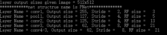
print ("Layer Name = %s, Output size = %3d, Stride = %3d, RF size = %3d" % (net_struct[net]['name'][i], p[0], p[1], rf))
Results are as follows
in addition calculated by the formula, there may be a more convenient way for manual calculation. Here are a few rules:
- Receptive fields initial layer is 1 featuremap
- Each layer through a convolution convkxk s1 (convolution kernel of size k, step size 1), receptive fields r = r + (k - 1), k = 3 common receptor field r = r + 2, k = 5 feel wild r = r + 4
- Each through a convolution layer or convkxk s2 max / avg pooling layer, receptive field r = (rx 2) + (k -2), conventional convolution kernel k = 3, s = 2, the receptive field r = rx 2 + 1, the convolution kernel k = 7, s = 2, the receptive field r = rx 2 + 5
- Maxpool2x2 s2 every elapse of a max / avg pooling downsampling layer receptive field r = rx 2
- After conv1x1 s1, ReLU, BN, dropout and other elements does not change the operation stage receptive field
- GAP layer after layer, and FC, the entire input image is receptive field
- Global step size is equal to step through all the layers of the multiplicative
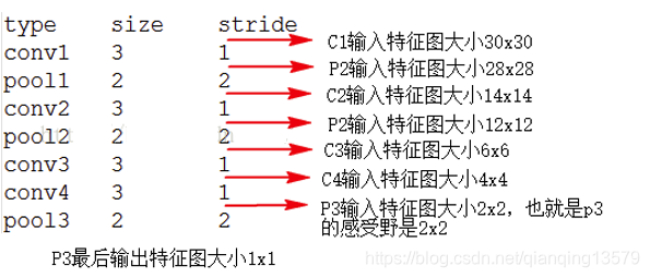
Specifically, when calculated using the bottom-up manner.
To calculate which layer the receptive field, is provided on the output layer is 1, and then successively calculates forward, such as the network structure in FIG, to calculate pool3 receptive field, the output of the pool3 set to 1, can be obtained conv1 input size 30x30, i.e. P3 receptive field size is 30.
According to this algorithm, we calculated the theoretical SSD300 in conv4-3 receptive fields:
R & lt = (((. 1 +2 + 2 + 2 + 2) X2 + 2 + 2 + 2) X2 + 2 + 2) X2 +2+ 2 = 108
NOTE: for the latter conv4-3 received a 3x3 convolution kernel regression and classification do so in the calculation of the size of the receptive field, needs to be used for classification and regression of the convolution kernel 3x3 is also taken into account.
Classic SSD network anchor setting
Classic network anchor size Here we look at how to set

Wherein the number in () represents: anchor / receptive field theory , this value is used hereinafter represents the size of the anchor.
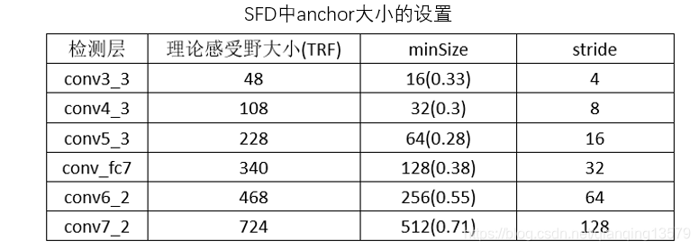
Note: SFD: Single Shot Scale-invariant Face Detector
The teacher open detector: ShiqiYu / libfacedetection in anchor setting
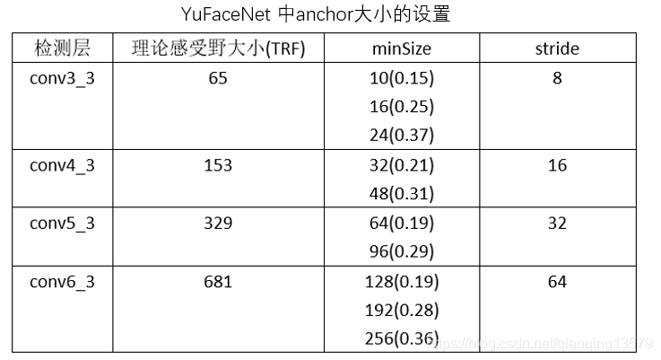

观察SSD,SFD,YuFace,RPN中的anchor设计,我们可以看出anchor的大小基本在[0.1,0.7]之间。RPN网络比较特别,anchor的大小超出了感受野大小。
anchor大小的探索
下面我做了一系列实验探索anchor大小的范围,分别在数据集A和数据集B上,使用SFD_VGG16和SSD_YuFaceNet两个模型,所有层的anchor大小分别设计为0.1~0.9,观察模型的AP和loss大小。
注:SFD_VGG16和SSD_YuFaceNet分别使用的是SFD开源的网络和ShiqiYu/libfacedetection开源的网络
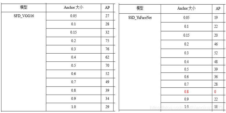
AP
数据集A:
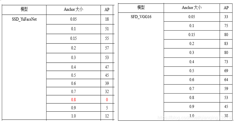
数据集B:
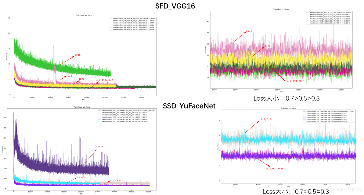
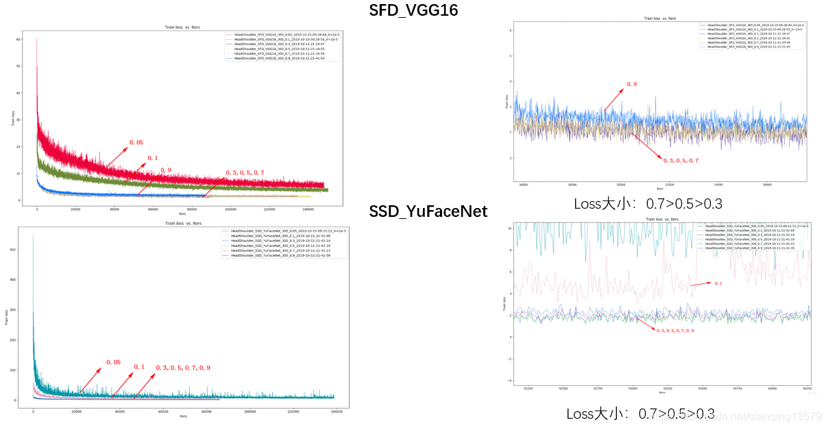
loss
数据集A:
数据集B:
实验分析
通过对经典网络的分析,以及实验的结果,可以观察到以下现象:
- anchor可以设置的范围较大,从实验结果来看,0.05~1.0基本都可以收敛,这也解释了为什么FasterRCNN中的RPN网络anchor大小可以超过感受野。从loss来看,anchor太大或者大小收敛效果都不好,甚至会出现不收敛的情况。这一点也很好理解,如果anchor太大,导致目标上下文信息较少,而如果anchor太小,又会导致没有足够多的信息。
- 综合AP的值以及loss的大小,我们可以看出,anchor在0.2~0.7之间收敛效果较好,这个结论与SSD经典网络的设置基本一致。这个范围既可以保证目标有足够多的上下文信息,也不会因为目标太小没有足够多的信息。
注:由于目前实验数据还不够充分,这个范围可能并不准确,欢迎大家留言讨论。
滑动窗口,感受野与anchor的关系
首先区分一下这几个比较容易混淆的概念:
- 滑动窗口:使得某一层输出大小为1的输入大小就是该层的滑动窗口大小。比如MTCNN中PNet,滑动窗口大小为12x12
- 理论感受野:影响某个神经元输出的输入区域,也就是该层能够感知到的区域
- 有效感受野:理论感受野中间对输出有重要影响的区域
- anchor:预先设置的每一层实际响应的区域
滑动窗口大小和理论感受野是一个网络的固有属性,一旦网络结构确定了,这两个参数就确定了,有效感受野是可以通过训练改变的,anchor是通过人工手动设置的。理论感受野,有效感受野,滑动窗口是对齐的, anchor设置过程中也要与感受野对齐,否则会影响检测效果。检测层上每个像素点都会对应一个理论感受野,滑动窗口以及anchor。
MTCNN中的anchor机制
MTCNN训练机制的问题
熟悉MTCNN的朋友应该都知道,训练MTCNN的时候需要事先生成三类样本:positive,part,negative.这三类样本是根据groundtruth的IOU来区分的,原论文中的设置是IOU<0.3的为negative,IOU>0.65的为positve,0.4<IOU<0.65的为part。
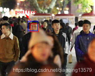
上图中生成的positive样本为,图中红色框为groundtruth,蓝色框为候选框

其中回归任务回归的就是两者之间的offset

回归的4个偏移量(公式不唯一):
对于小目标或者类似头肩这种目标,会出现一些问题
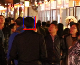
生成的positive样本如下:

基本上是一块黑色区域,没有太多有效信息。
对于小目标:
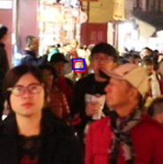
生成的positive是

这样的图像,这些图像是非常不利于训练的,而且MTCNN在训练的时候输入分辨率都比较小(比如12,24,48),将这些生成的图像resize到12,24或者48之后会导致有效信息更少,为了解决这个问题,我们需要包含目标更多的上下文信息,会更加容易识别。
MTCNN中的anchor机制
借鉴SSD中anchor的思想,提出了MTCNN中的anchor
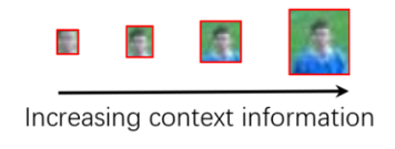
SSD在训练过程中通过anchor与groundtruth的匹配来确定每一个anchor的类别,具体匹配过程:计算与每个anchor的IOU最大(>阈值)的那个groundtruth,如果找到了,那么该anchor就匹配到了这个groundtruth,该anchor就是positive样本,anchor的类别就是该groundtruth的类别,回归的offset就是anchor与groundtruth之间的偏移量。由于SSD的anchor通常都比理论感受野小,所以SSD会包含较多的上下文信息,如下图所示。

联想到MTCNN,在生成训练样本的时候,我们可以将候选框当成anchor,生成positive的过程就是SSD中的匹配过程,由于需要包含更多上下文信息,最后会对anchor进行扩边生成最后的训练样本 。
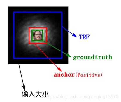
红色区域就是anchor也就是生成的positive样本,整个黑色区域就是对anchor做扩边后生成的训练样本,可以看到包含了更多的上下文信息。
实验结果与分析
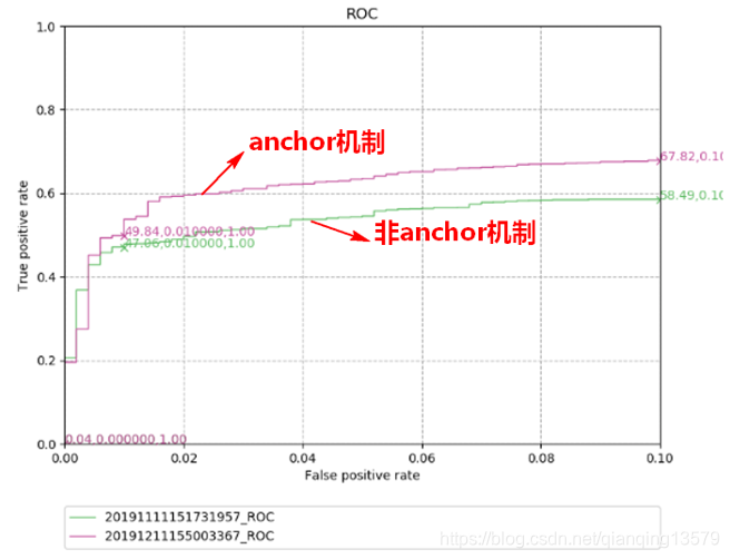
在多种数据集上对anchor机制进行了实验。
数据集1:
数据集2: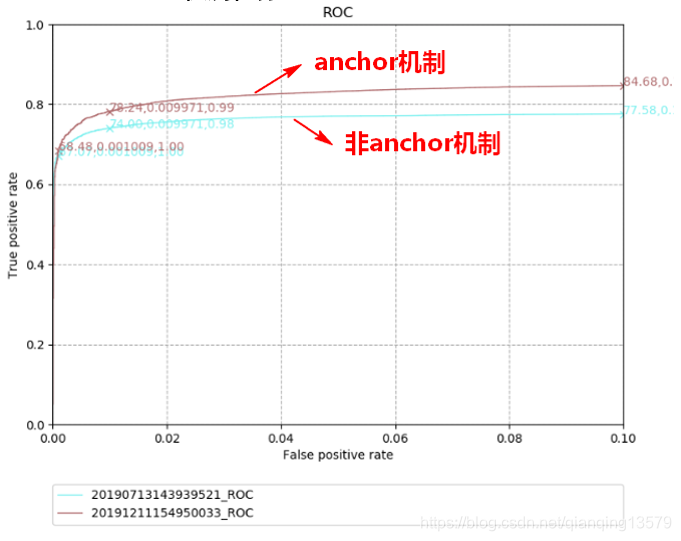
从实验结果我们可以看出,anchor机制可以显著提高检测器的精度。
结束语
关于anchor其实还有很多地方值得探索,本文只是总结了一下最近工作中对anchor的一些最新的认识,就当抛砖引玉,大家如果有关于anchor更好的解读欢迎一起讨论。
非常感谢您的阅读,如果您觉得这篇文章对您有帮助,欢迎扫码进行赞赏。
