Series blog, the original author maintained on GitHub: https://aka.ms/beginnerAI , click on the star with a star do not mean more stars the harder the author
Chapter 4 SISO single layer neural network
4.0 Univariate linear regression problem
4.0.1 Ask a question
In the early construction of the Internet, operators need to address the major problem is to ensure that the temperature of the room where the server perennial maintained at around 23 degrees Celsius. In a new room, if you plan to deploy 346 servers, how do we configure the maximum air-conditioning power?
Although this problem can calculate the thermodynamic equation, but there will always be errors. Thus people tend to install a thermostat in the engine room, the air conditioner switch or to control the rotational speed of the fan or cooling capacity, wherein the maximum cooling capacity is a critical value. More advanced approach is built directly on the seabed room, temperature reduction in the air isolated manner to the cooling water circulation.
By some statistics (referred to as sample data), we get Table 4-1.
Table 4-1 sample data
| Sample number | The number of servers (thousand units) X | Air conditioning Power (kW) Y |
|---|---|---|
| 1 | 0.928 | 4.824 |
| 2 | 0.469 | 2.950 |
| 3 | 0.855 | 4.643 |
| ... | ... | ... |
In the above samples, we generally referred to as the independent variable X sample characteristic value, referred to as the dependent variable Y sample value tag.
This data is two-dimensional, so we can use the visualization to show the way, the abscissa is the number of servers, the ordinate is the air conditioning power, shown in Figure 4-1.
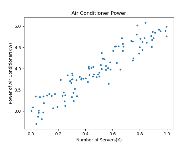
Figure 4-1 Sample Data Visualization
By observation of the figure, we can determine whether it belongs to a linear regression, and is the most simple linear regression. Thus, we have the problem of the thermodynamic calculations converted into a statistical problem, because it can not be accurately calculated or each board in the end of each machine can produce much heat.
Shrewd reader may think of a way: the sample data, we find a very similar case with the 346, with its reference to find the appropriate value of the air-conditioning power.
Have to admit, this is completely scientific and reasonable, in fact, this is the linear regression problem-solving ideas: the use of existing values, predict unknown values. In other words, these readers inadvertently used a linear regression model. In fact, this example is very simple, there is only one independent variable and one dependent variable, so you can use simple and direct method to solve the problem. However, when there are multiple arguments, this direct approach might ineffective. Suppose there are three independent variables, most likely not be able to find and combinations of these three arguments very close to the data in the sample, then we should make use of a more systematic approach.
4.0.2 linear regression model
Regression analysis is a mathematical model. When the independent variables and the dependent variable is a linear relationship, which is a particular linear model.
The simplest case is a linear regression, one argument of a substantially linear relationship between a dependent variable and the composition of the model are:
\ [Y = a + bX + ε \ tag {1} \]
X is the independent variable, Y is the dependent variable, ε is a random error, a and b are parameters of the linear regression model, a and b are we to learn out by the algorithm.
What is the model? When the first contact with this concept, there may be some unknown sleep Li. From conventional Conceptually, it is to constitute a description of the objective things by means of physical or virtual representation of subjective consciousness, this description usually there is a certain logic or mathematical meaning of abstract expression.
For example, model cars, it will be described: a four-wheel driven by the engine sub steel. Then it is the famous Einstein's special relativity inferences Energy Concept Modeling: \ (E = mc ^ 2 \) .
Modeling the data, then, is to find ways using one or more equations to describe the generation condition data, or relationships, such as a set of data substantially satisfies \ (y = 3x + 2 \ ) of this formula, then the formula is model. Why are said to be "substantially" mean? Because in the real world, in general, noise (error) exists, it is not possible to meet this very accurate formula, as long as this line is in the vicinity of both sides, it can be counted to meet the conditions.
For linear regression model, there are some concepts need to know the following:
- Random errors often assumed to mean 0 and variance σ ^ 2 (σ ^ 2> 0, σ ^ 2 regardless of the value of X)
- If it is further assumed to comply with normal random error, called the normal linear model
- Generally, if k independent variables and one dependent variable (i.e., the Y in Formula 1), due to the value of the variable is divided into two parts: the influence by an argument, it means that a function, a function of known form and unknown parameters; another portion of the other non-randomness and considerations, i.e., random errors
- When the function is a linear function of unknown parameters, called a linear regression model
- When the function is unknown parameter nonlinear function, called nonlinear regression analysis model
- When the number of arguments is greater than 1 is called multivariate regression
- When the number of the dependent variable is greater than 1 is called multiple regression
We observe the data, it can be broadly considered eligible linear regression model, so the list of Formula 1, without considering the random error, then our task is to find the right a and b, which is linear regression task.
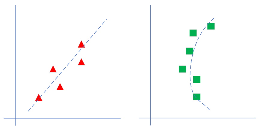
FIG distinction 4-2 linear regression and non-linear regression
Shown in Figure 4-2, the left linear model, it can be seen a straight line passing through the centerline region formed by a set of triangles, which does not require a straight line passing through each triangle. Right side is a nonlinear model, a curve passing through the centerline region of a set of rectangles is formed. In this chapter, we first learn how to solve the problem on the left side of the linear regression.
We will use the next several ways to solve this problem:
- Least squares;
- Gradient descent method;
- Simple neural network method;
- A more general neural network algorithm.
4.0.3 form formula
Here to explain the order of linear equations w and x. In many textbooks, we can see the following formula:
\ [Y = w ^ Tx + b \ {1} \]
or:
\[y = w \cdot x + b \tag{2}\]
And we use in this book:
\[y = x \cdot w + b \tag{3}\]
The main difference is the shape of the three sample data x is defined, correspondingly affect the definition of the shape of w. For example, if there are three feature value x, then w must have three weight values corresponding to the feature value, then:
Formula 1 in the form of a matrix
x is a column vector:
\[ x= \begin{pmatrix} x_{1} \\ x_{2} \\ x_{3} \end{pmatrix} \]
w is a column vector:
\[ w= \begin{pmatrix} w_{1} \\ w_{2} \\ w_{3} \end{pmatrix} \]
\[ y=w^Tx+b= \begin{pmatrix} w_1 & w_2 & w_3 \end{pmatrix} \begin{pmatrix} x_{1} \\ x_{2} \\ x_{3} \end{pmatrix} +b \]
\[ =w_1 \cdot x_1 + w_2 \cdot x_2 + w_3 \cdot x_3 + b \tag{4} \]
w和x都是列向量,所以需要先把w转置后,再与x做矩阵乘法。
公式2的矩阵形式
公式2与公式1的区别是w的形状,在公式2中,w直接就是个行向量:
\[ w= \begin{pmatrix} w_{1} & w_{2} & w_{3} \end{pmatrix} \]
而x的形状仍然是列向量:
\[ x= \begin{pmatrix} x_{1} \\ x_{2} \\ x_{3} \end{pmatrix} \]
这样相乘之前不需要做矩阵转置了:
\[ y=wx+b= \begin{pmatrix} w_1 & w_2 & w_3 \end{pmatrix} \begin{pmatrix} x_{1} \\ x_{2} \\ x_{3} \end{pmatrix} +b \]
\[ =w_1 \cdot x_1 + w_2 \cdot x_2 + w_3 \cdot x_3 + b \tag{5} \]
公式3的矩阵形式
x是个行向量:
\[ x= \begin{pmatrix} x_{1} & x_{2} & x_{3} \end{pmatrix} \]
w是列向量:
\[ w= \begin{pmatrix} w_{1} \\ w_{2} \\ x_{3} \end{pmatrix} \]
所以x在前,w在后:
\[ y=x \cdot w+b= \begin{pmatrix} x_1 & x_2 & x_3 \end{pmatrix} \begin{pmatrix} w_{1} \\ w_{2} \\ w_{3} \end{pmatrix} +b \]
\[ =x_1 \cdot w_1 + x_2 \cdot w_2 + x_3 \cdot w_3 + b \tag{6} \]
比较公式4,5,6,其实最后的运算结果是相同的。
我们再分析一下前两种形式的x矩阵,由于x是个列向量,意味着特征由行表示,当有2个样本同时参与计算时,x需要增加一列,变成了如下形式:
\[ x= \begin{pmatrix} x_{11} & x_{21} \\ x_{12} & x_{22} \\ x_{13} & x_{23} \end{pmatrix} \]
x的第一个下标表示样本序号,第二个下标表示样本特征,所以\(x_{21}\)是第2个样本的第1个特征。看\(x_{21}\)这个序号很别扭,一般我们都是认为行在前、列在后,但是\(x_{21}\)却是处于第1行第2列,和习惯正好相反。
如果采用第三种形式,则两个样本的x的矩阵是:
\[ x= \begin{pmatrix} x_{11} & x_{12} & x_{13} \\ x_{21} & x_{22} & x_{23} \end{pmatrix} \]
第1行是第1个样本的3个特征,第2行是第2个样本的3个特征,这与常用的阅读习惯正好一致,第1个样本的第2个特征在矩阵的第1行第2列,因此我们在本书中一律使用第三种形式来描述线性方程。
另外一个原因是,在很多深度学习库的实现中,确实是把x放在w前面做矩阵运算的,同时w的形状也是从左向右看,比如左侧有2个样本的3个特征输入(2x3表示2个样本3个特征值),右侧是1个输出,则w的形状就是3x1。否则的话就需要倒着看,w的形状成为了1x3,而x变成了3x2,很别扭。
对于b来说,它永远是1行,列数与w的列数相等。比如w是3x1的矩阵,则b是1x1的矩阵。如果w是3x2的矩阵,意味着3个特征输入到2个神经元上,则b是1x2的矩阵,每个神经元分配1个bias。
4.1 最小二乘法
4.1.1 历史
最小二乘法,也叫做最小平方法(Least Square),它通过最小化误差的平方和寻找数据的最佳函数匹配。利用最小二乘法可以简便地求得未知的数据,并使得这些求得的数据与实际数据之间误差的平方和为最小。最小二乘法还可用于曲线拟合。其他一些优化问题也可通过最小化能量或最小二乘法来表达。
1801年,意大利天文学家朱赛普·皮亚齐发现了第一颗小行星谷神星。经过40天的跟踪观测后,由于谷神星运行至太阳背后,使得皮亚齐失去了谷神星的位置。随后全世界的科学家利用皮亚齐的观测数据开始寻找谷神星,但是根据大多数人计算的结果来寻找谷神星都没有结果。时年24岁的高斯也计算了谷神星的轨道。奥地利天文学家海因里希·奥尔伯斯根据高斯计算出来的轨道重新发现了谷神星。
高斯使用的最小二乘法的方法发表于1809年他的著作《天体运动论》中。法国科学家勒让德于1806年独立发明“最小二乘法”,但因不为世人所知而默默无闻。勒让德曾与高斯为谁最早创立最小二乘法原理发生争执。
1829年,高斯提供了最小二乘法的优化效果强于其他方法的证明,因此被称为高斯-马尔可夫定理。
4.1.2 数学原理
线性回归试图学得:
\[z(x_i)=w \cdot x_i+b \tag{1}\]
使得:
\[z(x_i) \simeq y_i \tag{2}\]
其中,\(x_i\)是样本特征值,\(y_i\)是样本标签值,\(z_i\)是模型预测值。
如何学得w和b呢?均方差(MSE - mean squared error)是回归任务中常用的手段:
\[ J = \sum_{i=1}^m(z(x_i)-y_i)^2 = \sum_{i=1}^m(y_i-wx_i-b)^2 \tag{3} \]
\(J\)称为损失函数。实际上就是试图找到一条直线,使所有样本到直线上的残差的平方和最小。

图4-3 均方差函数的评估原理
图4-3中,圆形点是样本点,直线是当前的拟合结果。如左图所示,我们是要计算样本点到直线的垂直距离,需要再根据直线的斜率来求垂足然后再计算距离,这样计算起来很慢;但实际上,在工程上我们通常使用的是右图的方式,即样本点到直线的竖直距离,因为这样计算很方便,用一个减法就可以了。
假设我们计算出初步的结果是虚线所示,这条直线是否合适呢?我们来计算一下图中每个点到这条直线的距离,把这些距离的值都加起来(都是正数,不存在互相抵消的问题)成为误差。
因为上图中的几个点不在一条直线上,所以不能有一条直线能同时穿过它们。所以,我们只能想办法不断改变红色直线的角度和位置,让总体误差最小(用于不可能是0),就意味着整体偏差最小,那么最终的那条直线就是我们要的结果。
如果想让误差的值最小,通过对w和b求导,再令导数为0(到达最小极值),就是w和b的最优解。
推导过程如下:
\[ \begin{aligned} {\partial{J} \over \partial{w}} &={\partial{(\sum_{i=1}^m(y_i-wx_i-b)^2)} \over \partial{w}} \\ &= 2\sum_{i=1}^m(y_i-wx_i-b)(-x_i) \end{aligned} \tag{4} \]
令公式4为0:
\[ \sum_{i=1}^m(y_i-wx_i-b)x_i=0 \tag{5} \]
\[ \begin{aligned} {\partial{J} \over \partial{b}} &={\partial{(\sum_{i=1}^m(y_i-wx_i-b)^2)} \over \partial{b}} \\ &=2\sum_{i=1}^m(y_i-wx_i-b)(-1) \end{aligned} \tag{6} \]
令公式6为0:
\[ \sum_{i=1}^m(y_i-wx_i-b)=0 \tag{7} \]
由式7得到(假设有m个样本):
\[ \sum_{i=1}^m b = m \cdot b = \sum_{i=1}^m{y_i} - w\sum_{i=1}^m{x_i} \tag{8} \]
两边除以m:
\[ b = {1 \over m}(\sum_{i=1}^m{y_i} - w\sum_{i=1}^m{x_i})=\bar y-w \bar x \tag{9} \]
其中:
\[ \bar y = {1 \over m}\sum_{i=1}^m y_i, \bar x={1 \over m}\sum_{i=1}^m x_i \tag{10} \]
将公式10代入公式5:
\[ \sum_{i=1}^m(y_i-wx_i-\bar y + w \bar x)x_i=0 \]
\[ \sum_{i=1}^m(x_i y_i-wx^2_i-x_i \bar y + w \bar x x_i)=0 \]
\[ \sum_{i=1}^m(x_iy_i-x_i \bar y)-w\sum_{i=1}^m(x^2_i - \bar x x_i) = 0 \]
\[ w = {\sum_{i=1}^m(x_iy_i-x_i \bar y) \over \sum_{i=1}^m(x^2_i - \bar x x_i)} \tag{11} \]
将公式10代入公式11:
\[ w={\sum_{i=1}^m (x_i \cdot y_i) - \sum_{i=1}^m x_i \cdot {1 \over m} \sum_{i=1}^m y_i \over \sum_{i=1}^m x^2_i - \sum_{i=1}^m x_i \cdot {1 \over m}\sum_{i=1}^m x_i} \tag{12} \]
分子分母都乘以m:
\[ w={m\sum_{i=1}^m x_i y_i - \sum_{i=1}^m x_i \sum_{i=1}^m y_i \over m\sum_{i=1}^m x^2_i - (\sum_{i=1}^m x_i)^2} \tag{13} \]
\[ b=\frac{1}{m}\sum_{i=1}^m(y_i-wx_i) \tag{14} \]
而事实上,式13有很多个变种,大家会在不同的文章里看到不同版本,往往感到困惑,比如下面两个公式也是正确的解:
\[ w = {\sum_{i=1}^m y_i(x_i-\bar x) \over \sum_{i=1}^m x^2_i - (\sum_{i=1}^m x_i)^2/m} \tag{15} \]
\[ w = {\sum_{i=1}^m x_i(y_i-\bar y) \over \sum_{i=1}^m x^2_i - \bar x \sum_{i=1}^m x_i} \tag{16} \]
以上两个公式,如果把公式10代入,也应该可以得到和式13相同的答案,只不过需要一些运算技巧。比如,很多人不知道这个神奇的公式:
\[ \begin{aligned} \sum_{i=1}^m (x_i \bar y) &= \bar y \sum_{i=1}^m x_i =\frac{1}{m}(\sum_{i=1}^m y_i) (\sum_{i=1}^m x_i) \\ &=\frac{1}{m}(\sum_{i=1}^m x_i) (\sum_{i=1}^m y_i)= \bar x \sum_{i=1}^m y_i \\ &=\sum_{i=1}^m (y_i \bar x) \end{aligned} \tag{17} \]
4.1.3 代码实现
我们下面用Python代码来实现一下以上的计算过程:
计算w值
# 根据公式15
def method1(X,Y,m):
    x_mean = X.mean()
    p = sum(Y*(X-x_mean))
    q = sum(X*X) - sum(X)*sum(X)/m
    w = p/q
    return w

# 根据公式16
def method2(X,Y,m):
    x_mean = X.mean()
    y_mean = Y.mean()
    p = sum(X*(Y-y_mean))
    q = sum(X*X) - x_mean*sum(X)
    w = p/q
    return w

# 根据公式13
def method3(X,Y,m):
    p = m*sum(X*Y) - sum(X)*sum(Y)
    q = m*sum(X*X) - sum(X)*sum(X)
    w = p/q
    return w
由于有函数库的帮助,我们不需要手动计算sum(), mean()这样的基本函数。
计算b值
# 根据公式14
def calculate_b_1(X,Y,w,m):
    b = sum(Y-w*X)/m
    return b

# 根据公式9
def calculate_b_2(X,Y,w):
    b = Y.mean() - w * X.mean()
    return b
4.1.4 运算结果
用以上几种方法,最后得出的结果都是一致的,可以起到交叉验证的作用:
w1=2.056827, b1=2.965434
w2=2.056827, b2=2.965434
w3=2.056827, b3=2.965434
代码位置
ch04, Level1
4.2 梯度下降法
有了上一节的最小二乘法做基准,我们这次用梯度下降法求解w和b,从而可以比较二者的结果。
4.2.1 数学原理
在下面的公式中,我们规定x是样本特征值(单特征),y是样本标签值,z是预测值,下标 \(i\) 表示其中一个样本。
预设函数(Hypothesis Function)
为一个线性函数:
\[z_i = x_i \cdot w + b \tag{1}\]
损失函数(Loss Function)
为均方差函数:
\[loss(w,b) = \frac{1}{2} (z_i-y_i)^2 \tag{2}\]
与最小二乘法比较可以看到,梯度下降法和最小二乘法的模型及损失函数是相同的,都是一个线性模型加均方差损失函数,模型用于拟合,损失函数用于评估效果。
区别在于,最小二乘法从损失函数求导,直接求得数学解析解,而梯度下降以及后面的神经网络,都是利用导数传递误差,再通过迭代方式一步一步(用近似解)逼近真实解。
4.2.2 梯度计算
计算z的梯度
根据公式2:
\[ {\partial loss \over \partial z_i}=z_i - y_i \tag{3} \]
计算w的梯度
我们用loss的值作为误差衡量标准,通过求w对它的影响,也就是loss对w的偏导数,来得到w的梯度。由于loss是通过公式2->公式1间接地联系到w的,所以我们使用链式求导法则,通过单个样本来求导。
根据公式1和公式3:
\[ {\partial{loss} \over \partial{w}} = \frac{\partial{loss}}{\partial{z_i}}\frac{\partial{z_i}}{\partial{w}}=(z_i-y_i)x_i \tag{4} \]
计算b的梯度
\[ \frac{\partial{loss}}{\partial{b}} = \frac{\partial{loss}}{\partial{z_i}}\frac{\partial{z_i}}{\partial{b}}=z_i-y_i \tag{5} \]
4.2.3 代码实现
if __name__ == '__main__':

    reader = SimpleDataReader()
    reader.ReadData()
    X,Y = reader.GetWholeTrainSamples()

    eta = 0.1
    w, b = 0.0, 0.0
    for i in range(reader.num_train):
        # get x and y value for one sample
        xi = X[i]
        yi = Y[i]
        # 公式1
        zi = xi * w + b
        # 公式3
        dz = zi - yi
        # 公式4
        dw = dz * xi
        # 公式5
        db = dz
        # update w,b
        w = w - eta * dw
        b = b - eta * db

    print("w=", w)
    print("b=", b)
大家可以看到,在代码中,我们完全按照公式推导实现了代码,所以,大名鼎鼎的梯度下降,其实就是把推导的结果转化为数学公式和代码,直接放在迭代过程里!另外,我们并没有直接计算损失函数值,而只是把它融入在公式推导中。
4.2.4 运行结果
w= [1.71629006]
b= [3.19684087]
读者可能会注意到,上面的结果和最小二乘法的结果(w1=2.056827, b1=2.965434)相差比较多,这个问题我们留在本章稍后的地方解决。
代码位置
ch04, Level2
4.3 神经网络法
在梯度下降法中,我们简单讲述了一下神经网络做线性拟合的原理,即:
- 初始化权重值
- 根据权重值放出一个解
- 根据均方差函数求误差
- 误差反向传播给线性计算部分以调整权重值
- 是否满足终止条件?不满足的话跳回2
一个不恰当的比喻就是穿糖葫芦:桌子上放了一溜儿12个红果,给你一个足够长的竹签子,选定一个角度,在不移动红果的前提下,想办法用竹签子穿起最多的红果。
最开始你可能会任意选一个方向,用竹签子比划一下,数数能穿到几个红果,发现是5个;然后调整一下竹签子在桌面上的水平角度,发现能穿到6个......最终你找到了能穿10个红果的的角度。
4.3.1 定义神经网络结构
我们是首次尝试建立神经网络,先用一个最简单的单层单点神经元,如图4-4所示。

图4-4 单层单点神经元
下面,我们用这个最简单的线性回归的例子,来说明神经网络中最重要的反向传播和梯度下降的概念、过程以及代码实现。
输入层
此神经元在输入层只接受一个输入特征,经过参数w,b的计算后,直接输出结果。这样一个简单的“网络”,只能解决简单的一元线性回归问题,而且由于是线性的,我们不需要定义激活函数,这就大大简化了程序,而且便于大家循序渐进地理解各种知识点。
严格来说输入层在神经网络中并不能称为一个层。
权重w/b
因为是一元线性问题,所以w/b都是一个标量。
输出层
输出层1个神经元,线性预测公式是:
\[z_i = x_i \cdot w + b\]
z是模型的预测输出,y是实际的样本标签值,下标 \(i\) 为样本。
损失函数
因为是线性回归问题,所以损失函数使用均方差函数。
\[loss(w,b) = \frac{1}{2} (z_i-y_i)^2\]
4.3.2 反向传播
由于我们使用了和上一节中的梯度下降法同样的数学原理,所以反向传播的算法也是一样的,细节请查看4.2.2。
计算w的梯度
\[ {\partial{loss} \over \partial{w}} = \frac{\partial{loss}}{\partial{z_i}}\frac{\partial{z_i}}{\partial{w}}=(z_i-y_i)x_i \]
计算b的梯度
\[ \frac{\partial{loss}}{\partial{b}} = \frac{\partial{loss}}{\partial{z_i}}\frac{\partial{z_i}}{\partial{b}}=z_i-y_i \]
为了简化问题,在本小节中,反向传播使用单样本方式,在下一小节中,我们将介绍多样本方式。
4.3.3 代码实现
其实神经网络法和梯度下降法在本质上是一样的,只不过神经网络法使用一个崭新的编程模型,即以神经元为中心的代码结构设计,这样便于以后的功能扩充。
在Python中可以使用面向对象的技术,通过创建一个类来描述神经网络的属性和行为,下面我们将会创建一个叫做NeuralNet的class,然后通过逐步向此类中添加方法,来实现神经网络的训练和推理过程。
定义类
class NeuralNet(object):
    def __init__(self, eta):
        self.eta = eta
        self.w = 0
        self.b = 0
NeuralNet类从object类派生,并具有初始化函数,其参数是eta,也就是学习率,需要调用者指定。另外两个成员变量是w和b,初始化为0。
前向计算
    def __forward(self, x):
        z = x * self.w + self.b
        return z
这是一个私有方法,所以前面有两个下划线,只在NeuralNet类中被调用,不对外公开。
反向传播
下面的代码是通过梯度下降法中的公式推导而得的,也设计成私有方法:
    def __backward(self, x,y,z):
        dz = z - y
        db = dz
        dw = x * dz
        return dw, db
dz是中间变量,避免重复计算。dz又可以写成delta_Z,是当前层神经网络的反向误差输入。
梯度更新
    def __update(self, dw, db):
        self.w = self.w - self.eta * dw
        self.b = self.b - self.eta * db
每次更新好新的w和b的值以后,直接存储在成员变量中,方便下次迭代时直接使用,不需要在全局范围当作参数内传来传去的。
训练过程
只训练一轮的算法是:
for 循环,直到所有样本数据使用完毕:
- 读取一个样本数据
- 前向计算
- 反向传播
- 更新梯度
    def train(self, dataReader):
        for i in range(dataReader.num_train):
            # get x and y value for one sample
            x,y = dataReader.GetSingleTrainSample(i)
            # get z from x,y
            z = self.__forward(x)
            # calculate gradient of w and b
            dw, db = self.__backward(x, y, z)
            # update w,b
            self.__update(dw, db)
        # end for
推理预测
    def inference(self, x):
        return self.__forward(x)
推理过程,实际上就是一个前向计算过程,我们把它单独拿出来,方便对外接口的设计,所以这个方法被设计成了公开的方法。
主程序
if __name__ == '__main__':
    # read data
    sdr = SimpleDataReader()
    sdr.ReadData()
    # create net
    eta = 0.1
    net = NeuralNet(eta)
    net.train(sdr)
    # result
    print("w=%f,b=%f" %(net.w, net.b))
    # predication
    result = net.inference(0.346)
    print("result=", result)
    ShowResult(net, sdr)
4.3.4 运行结果可视化
打印输出结果:
w=1.716290,b=3.196841
result= [3.79067723]最终我们得到了W和B的值,对应的直线方程是\(y=1.71629x+3.196841\)。推理预测时,已知有346台服务器,先要除以1000,因为横坐标是以K(千台)服务器为单位的,代入前向计算函数,得到的结果是3.74千瓦。
结果显示函数:
def ShowResult(net, dataReader):
    ......
对于初学神经网络的人来说,可视化的训练过程及结果,可以极大地帮助理解神经网络的原理,Python的Matplotlib库提供了非常丰富的绘图功能。
在上面的函数中,先获得所有样本点数据,把它们绘制出来。然后在[0,1]之间等距设定10个点做为x值,用x值通过网络推理方法net.inference()获得每个点的y值,最后把这些点连起来,就可以画出图4-5中的拟合直线。
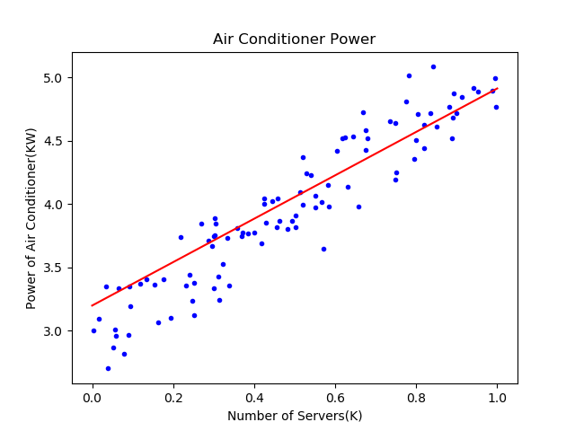
图4-5 拟合效果
可以看到红色直线虽然穿过了蓝色点阵,但是好像不是处于正中央的位置,应该再逆时针旋转几度才会达到最佳的位置。我们后面小节中会讲到如何提高训练结果的精度问题。
4.3.5 工作原理
就单纯地看待这个线性回归问题,其原理就是先假设样本点是呈线性分布的,注意这里的线性有可能是高维空间的,而不仅仅是二维平面上的。但是高维空间人类无法想象,所以我们不妨用二维平面上的问题来举例。
在4.2的梯度下降法中,首先假设这个问题是个线性问题,因而有了公式\(z=xw+b\),用梯度下降的方式求解最佳的\(w、b\)的值。
在本节中,用神经元的编程模型把梯度下降法包装了一下,这样就进入了神经网络的世界,从而可以有成熟的方法论可以解决更复杂的问题,比如多个神经元协同工作、多层神经网络的协同工作等等。
如图4-5所示,样本点摆在那里,位置都是固定的了,神经网络的任务就是找到一根直线(注意我们首先假设这是线性问题),让该直线穿过样本点阵,并且所有样本点到该直线的距离的平方的和最小。
可以想象成每一个样本点都有一根橡皮筋连接到直线上,连接点距离该样本点最近,所有的橡皮筋形成一个合力,不断地调整该直线的位置。该合力具备两种调节方式:
- 如果上方的拉力大一些,直线就会向上平移一些,这相当于调节b值;
- 如果侧方的拉力大一些,直线就会向侧方旋转一些,这相当于调节w值。
直到该直线处于平衡位置时,也就是线性拟合的最佳位置了。
如果样本点不是呈线性分布的,可以用直线拟合吗?
答案是“可以的”,只是最终的效果不太理想,误差可以做到在线性条件下的最小,但是误差值本身还是比较大的。比如一个半圆形的样本点阵,用直线拟合可以达到误差值最小为1.2(不妨假设这个值的单位是厘米),已经尽力了但能力有限。如果用弧线去拟合,可以达到误差值最小为0.3。
所以,当使用线性回归的效果不好时,即判断出一个问题不是线性问题时,我们会用第9章的方法来解决。
代码位置
ch04, Level3
思考和练习
- 请把上述代码中的dw和db也改成私有属性,然后试着运行程序。
4.4 多样本单特征值计算
在前面的代码中,我们一直使用单样本计算来实现神经网络的训练过程,但是单样本计算有一些缺点:
- 很有可能前后两个相邻的样本,会对反向传播产生相反的作用而互相抵消。假设样本1造成了误差为0.5,w的梯度计算结果是0.1;紧接着样本2造成的误差为-0.5,w的梯度计算结果是-0.1,那么前后两次更新w就会产生互相抵消的作用。
- 在样本数据量大时,逐个计算会花费很长的时间。由于我们在本例中样本量不大(200个样本),所以计算速度很快,觉察不到这一点。在实际的工程实践中,动辄10万甚至100万的数据量,轮询一次要花费很长的时间。
如果使用多样本计算,就要涉及到矩阵运算了,而所有的深度学习框架,都对矩阵运算做了优化,会大幅提升运算速度。打个比方:如果200个样本,循环计算一次需要2秒的话,那么把200个样本打包成矩阵,做一次计算也许只需要0.1秒。
下面我们来看看多样本运算会对代码实现有什么影响,假设我们一次用3个样本来参与计算,每个样本只有1个特征值。
4.4.1 前向计算
由于有多个样本同时计算,所以我们使用\(x_i\)表示第 \(i\) 个样本,X是样本组成的矩阵,Z是计算结果矩阵,w和b都是标量:
\[ Z = X \cdot w + b \tag{1} \]
把它展开成3个样本(3行,每行代表一个样本)的形式:
\[ X=\begin{pmatrix} x_1 \\ x_2 \\ x_3 \end{pmatrix} \]
\[ Z= \begin{pmatrix} x_1 \\ x_2 \\ x_3 \end{pmatrix} \cdot w + b = \begin{pmatrix} x_1 \cdot w + b \\ x_2 \cdot w + b \\ x_3 \cdot w + b \end{pmatrix} = \begin{pmatrix} z_1 \\ z_2 \\ z_3 \end{pmatrix} \tag{2} \]
\(z_1、z_2、z_3\)是三个样本的计算结果。根据公式1和公式2,我们的前向计算python代码可以写成:
    def __forwardBatch(self, batch_x):
        Z = np.dot(batch_x, self.w) + self.b
        return Z
Python中的矩阵乘法命名有些问题,np.dot()并不是矩阵点乘,而是矩阵叉乘,请读者习惯。
4.4.2 损失函数
用传统的均方差函数,其中,z是每一次迭代的预测输出,y是样本标签数据。我们使用m个样本参与计算,因此损失函数为:
\[J(w,b) = \frac{1}{2m}\sum_{i=1}^{m}(z_i - y_i)^2\]
其中的分母中有个2,实际上是想在求导数时把这个2约掉,没有什么原则上的区别。
我们假设每次有3个样本参与计算,即m=3,则损失函数实例化后的情形是:
\[ \begin{aligned} J(w,b) &= \frac{1}{2\times3}[(z_1-y_1)^2+(z_2-y_2)^2+(z_3-y_3)^2] \\ &=\frac{1}{2\times3}\sum_{i=1}^3[(z_i-y_i)^2] \\ \end{aligned} \tag{3} \]
公式3中大写的Z和Y都是矩阵形式,用代码实现:
    def __checkLoss(self, dataReader):
        X,Y = dataReader.GetWholeTrainSamples()
        m = X.shape[0]
        Z = self.__forwardBatch(X)
        LOSS = (Z - Y)**2
        loss = LOSS.sum()/m/2
        return loss
Python中的矩阵减法运算,不需要对矩阵中的每个对应的元素单独做减法,而是整个矩阵相减即可。做求和运算时,也不需要自己写代码做遍历每个元素,而是简单地调用求和函数即可。
4.4.3 求w的梯度
我们用 J 的值作为基准,去求 w 对它的影响,也就是 J 对 w 的偏导数,就可以得到w的梯度了。从公式3看 J 的计算过程,\(z_1、z_2、z_3\)都对它有贡献;再从公式2看\(z_1、z_2、z_3\)的生成过程,都有w的参与。所以,J 对 w 的偏导应该是这样的:
\[ \begin{aligned} \frac{\partial{J}}{\partial{w}}&=\frac{\partial{J}}{\partial{z_1}}\frac{\partial{z_1}}{\partial{w}}+\frac{\partial{J}}{\partial{z_2}}\frac{\partial{z_2}}{\partial{w}}+\frac{\partial{J}}{\partial{z_3}}\frac{\partial{z_3}}{\partial{w}} \\ &=\frac{1}{3}[(z_1-y_1)x_1+(z_2-y_2)x_2+(z_3-y_3)x_3] \\ &=\frac{1}{3} \begin{pmatrix} x_1 & x_2 & x_3 \end{pmatrix} \begin{pmatrix} z_1-y_1 \\ z_2-y_2 \\ z_3-y_3 \end{pmatrix} \\ &=\frac{1}{m} \sum^m_{i=1} (z_i-y_i)x_i \\ &=\frac{1}{m} X^T \cdot (Z-Y) \\ \end{aligned} \tag{4} \]
其中:
\[X = \begin{pmatrix} x_1 \\ x_2 \\ x_3 \end{pmatrix}, X^T = \begin{pmatrix} x_1 & x_2 & x_3 \end{pmatrix} \]
公式4中最后两个等式其实是等价的,只不过倒数第二个公式用求和方式计算每个样本,最后一个公式用矩阵方式做一次性计算。
4.4.4 求b的梯度
\[ \begin{aligned} \frac{\partial{J}}{\partial{b}}&=\frac{\partial{J}}{\partial{z_1}}\frac{\partial{z_1}}{\partial{b}}+\frac{\partial{J}}{\partial{z_2}}\frac{\partial{z_2}}{\partial{b}}+\frac{\partial{J}}{\partial{z_3}}\frac{\partial{z_3}}{\partial{b}} \\ &=\frac{1}{3}[(z_1-y_1)+(z_2-y_2)+(z_3-y_3)] \\ &=\frac{1}{m} \sum^m_{i=1} (z_i-y_i) \\ &=\frac{1}{m}(Z-Y) \end{aligned} \tag{5} \]
公式5中最后两个等式也是等价的,在python中,可以直接用最后一个公式求矩阵的和,免去了一个个计算\(z_i-y_i\)最后再求和的麻烦,速度还快。
    def __backwardBatch(self, batch_x, batch_y, batch_z):
        m = batch_x.shape[0]
        dZ = batch_z - batch_y
        dW = np.dot(batch_x.T, dZ)/m
        dB = dZ.sum(axis=0, keepdims=True)/m
        return dW, dB
代码位置
ch04, HelperClass/NeuralNet.py
4.5 梯度下降的三种形式
我们比较一下目前我们用三种方法得到的w和b的值,见表4-2。
表4-2 三种方法的结果比较
| 方法 | w | b |
|---|---|---|
| 最小二乘法 | 2.056827 | 2.965434 |
| 梯度下降法 | 1.71629006 | 3.19684087 |
| 神经网络法 | 1.71629006 | 3.19684087 |
这个问题的原始值是可能是\(w=2,b=3\),由于样本噪音的存在,使用最小二乘法得到了2.05、2.96这样的非整数解,这是完全可以接受的。但是使用梯度下降和神经网络两种方式,都得到1.71、3.19这样的值,准确程度很低。从图4-6的神经网络的训练结果来看,拟合直线是斜着穿过样本点区域的,并没有在正中央的骨架上。

图4-6 拟合效果
难度是神经网络方法有什么问题吗?
初次使用神经网络,一定有水土不服的地方。最小二乘法可以得到数学解析解,所以它的结果是可信的。梯度下降法和神经网络法实际是一回事儿,只是梯度下降没有使用神经元模型而已。所以,接下来我们研究一下如何调整神经网络的训练过程,先从最简单的梯度下降的三种形式说起。
在下面的说明中,我们使用如下假设,以便简化问题易于理解:
- 使用可以解决本章的问题的线性回归模型,即\(z=x \cdot w+b\)
- 样本特征值数量为1,即\(x、w、b\)都是标量
- 使用均方差损失函数。
计算w的梯度:
\[ {\partial{loss} \over \partial{w}} = \frac{\partial{loss}}{\partial{z_i}}\frac{\partial{z_i}}{\partial{w}}=(z_i-y_i)x_i \]
计算b的梯度:
\[ \frac{\partial{loss}}{\partial{b}} = \frac{\partial{loss}}{\partial{z_i}}\frac{\partial{z_i}}{\partial{b}}=z_i-y_i \]
4.5.1 单样本随机梯度下降
SDG(Stochastic Grident Descent)
样本访问示意图如图4-7所示。
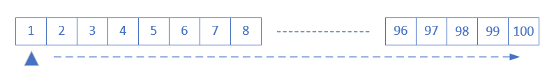
图4-7 单样本访问方式
计算过程
假设一共100个样本,每次使用1个样本:
\(repeat\{ \\\)
\(\quad for \quad i=1,2,3,...,100\{ \\\)
\(\quad \quad z_i = x_i \cdot w + b\\\)
\(\quad \quad dw= x_i \cdot (z_i - y_i)\\\)
\(\quad \quad db= z_i - y_i \\\)
\(\quad \quad w=w-\eta \cdot dw \\\)
\(\quad \quad db=b-\eta \cdot db \\\)
\(\quad\} \\\)
\(\}\)
特点
- 训练样本:每次使用一个样本数据进行一次训练,更新一次梯度,重复以上过程。
- 优点:训练开始时损失值下降很快,随机性大,找到最优解的可能性大。
- 缺点:受单个样本的影响最大,损失函数值波动大,到后期徘徊不前,在最优解附近震荡。不能并行计算。
运行结果
设置batch_size=1,即单样本方式:
if __name__ == '__main__':
    sdr = SimpleDataReader()
    sdr.ReadData()
    params = HyperParameters(1, 1, eta=0.1, max_epoch=100, batch_size=1, eps = 0.02)
    net = NeuralNet(params)
    net.train(sdr)
表4-3 单样本方式的训练情况
| 损失函数值 | 梯度下降过程 |
|---|---|
 |
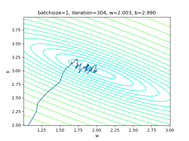 |
表4-3的左图,由于我们使用了限定的停止条件,即当损失函数值小于等于0.02时停止训练,所以,单样本方式迭代了300次后达到了精度要求。
右图是w和b共同构成的损失函数等高线图。梯度下降时,开始收敛较快,稍微有些弯曲地向中央地带靠近。到后期波动较大,找不到准确的前进方向,曲折地达到中心附近。
4.5.2 小批量样本梯度下降
Mini-Batch Gradient Descent
样本访问示意图如图4-8所示。
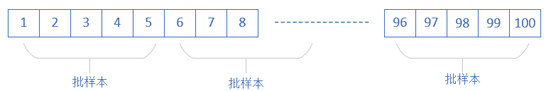
图4-8 小批量样本访问方式
计算过程
假设一共100个样本,每个小批量5个样本:
\(repeat\{ \\\)
\(\quad for \quad i=1,6,11,...,96\{\\\)
\(\quad \quad z_i = x_i \cdot w + b \\\)
\(\quad \quad z_{i+1} = x_{i+1} \cdot w + b \\\)
\(\quad \quad \dots \\\)
\(\quad \quad z_{i+4} = x_{i+4} \cdot w + b \\\)
\(\quad \quad dw= {1 \over 5}\sum_{k=i}^{i+4} x_k \cdot (z_k - y_k) \\\)
\(\quad \quad db= {1 \over 5}\sum_{k=i}^{i+4} (z_k - y_k) \\\)
\(\quad \quad w=w-\eta \cdot dw \\\)
\(\quad \quad db=b-\eta \cdot db \\\)
\(\quad\}\\\)
\(\}\)
上述算法中,循环体中的前5行分别计算了\(z_i, z_{i+1}, ..., z_{i+4}\),可以换成一次性的矩阵运算。
特点
- 训练样本:选择一小部分样本进行训练,更新一次梯度,然后再选取另外一小部分样本进行训练,再更新一次梯度。
- 优点:不受单样本噪声影响,训练速度较快。
- 缺点:batch size的数值选择很关键,会影响训练结果。
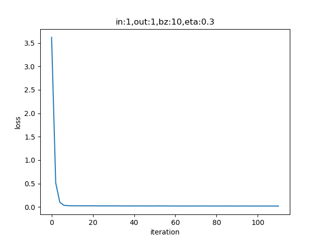
运行结果
设置batch_size=10:
if __name__ == '__main__':
    sdr = SimpleDataReader()
    sdr.ReadData()
    params = HyperParameters(1, 1, eta=0.3, max_epoch=100, batch_size=10, eps = 0.02)
    net = NeuralNet(params)
    net.train(sdr)
表4-4 小批量样本方式的训练情况
| 损失函数值 | 梯度下降过程 |
|---|---|
 |
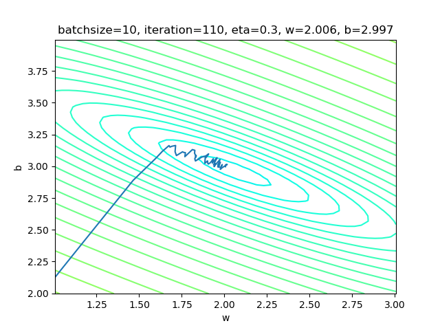 |
表4-4的右图,梯度下降时,在接近中心时有小波动。图太小看不清楚,可以用matplot工具放大局部来观察。和单样本方式比较,在中心区的波动已经缓解了很多。
小批量的大小通常由以下几个因素决定:
- 更大的批量会计算更精确的梯度,但是回报却是小于线性的。
- 极小批量通常难以充分利用多核架构。这决定了最小批量的数值,低于这个值的小批量处理不会减少计算时间。
- 如果批量处理中的所有样本可以并行地处理,那么内存消耗和批量大小成正比。对于多硬件设施,这是批量大小的限制因素。
- 某些硬件上使用特定大小的数组时,运行时间会更少,尤其是GPU,通常使用2的幂数作为批量大小可以更快,如32 ~ 256,大模型时尝试用16。
- 可能是由于小批量在学习过程中加入了噪声,会带来一些正则化的效果。泛化误差通常在批量大小为1时最好。因为梯度估计的高方差,小批量使用较小的学习率,以保持稳定性,但是降低学习率会使迭代次数增加。
在实际工程中,我们通常使用小批量梯度下降形式。
4.5.3 全批量样本梯度下降
Full Batch Gradient Descent
样本访问示意图如图4-9所示。
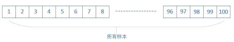
图4-9 全批量样本访问方式
计算过程
假设一共100个样本,每次使用全部样本:
\(repeat\{ \\\)
\(\quad z_1 = x_1 \cdot w + b \\\)
\(\quad z_2 = x_2 \cdot w + b \\\)
\(\quad \dots \\\)
\(\quad z_{100} = x_{100} \cdot w + b \\\)
\(\quad dw= {1 \over 100}\sum_{i=1}^{100} x_i \cdot (z_i - y_i) \\\)
\(\quad db= {1 \over 100}\sum_{i=1}^{100} (z_i - y_i) \\\)
\(\quad w=w-\eta \cdot dw \\\)
\(\quad db=b-\eta \cdot db \\\)
\(\}\)
上述算法中,循环体中的前100行分别计算了\(z_1, z_2, ..., z_{100}\),可以换成一次性的矩阵运算。
特点
- 训练样本:每次使用全部数据集进行一次训练,更新一次梯度,重复以上过程。
- 优点:受单个样本的影响最小,一次计算全体样本速度快,损失函数值没有波动,到达最优点平稳。方便并行计算。
- 缺点:数据量较大时不能实现(内存限制),训练过程变慢。初始值不同,可能导致获得局部最优解,并非全局最优解。
运行结果
if __name__ == '__main__':
    sdr = SimpleDataReader()
    sdr.ReadData()
    params = HyperParameters(1, 1, eta=0.5, max_epoch=1000, batch_size=-1, eps = 0.02)
    net = NeuralNet(params)
    net.train(sdr)
设置batch_size=-1,即是全批量的意思。
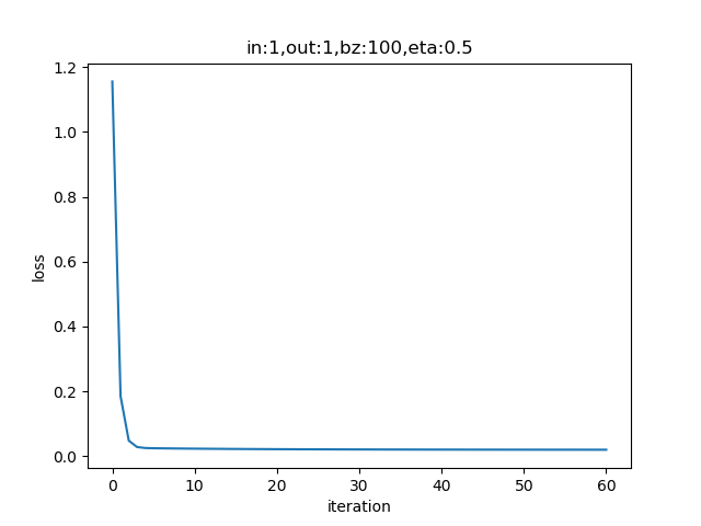
表4-5 全批量样本方式的训练情况
| 损失函数值 | 梯度下降过程 |
|---|---|
 |
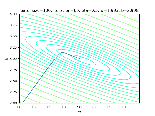 |
表4-5中的右图,梯度下降时,在整个过程中只拐了一个弯儿,就直接到达了中心点。
4.5.4 三种方式的比较
表4-6 三种方式的比较
| 单样本 | 小批量 | 全批量 | |
|---|---|---|---|
| 批大小 | 1 | 10 | 100 |
| 学习率 | 0.1 | 0.3 | 0.5 |
| 迭代次数 | 304 | 110 | 60 |
| epoch | 3 | 10 | 60 |
| 结果 | w=2.003, b=2.990 | w=2.006, b=2.997 | w=1.993, b=2.998 |
表4-6比较了三种方式的结果,从结果看,都接近于\(w=2,b=3\)的原始解。最后的可视化结果图如图4-10,可以看到直线已经处于样本点比较中间的位置。
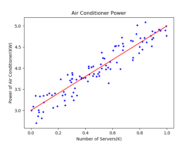
图4-10 较理想的拟合效果图
相关的概念:
- Batch Size:批大小,一次训练的样本数量。
- Iteration:迭代,一次正向 + 一次反向。
- Epoch:所有样本被使用了一次,叫做一个Epoch,中文的翻译比较杂乱,所以干脆就用原文比较清楚。
假设一共有样本1000个,batch size=20,则一个Epoch中,需要1000/20=50次Iteration才能训练完所有样本。
代码位置
ch04, Level5
思考与练习
- 调整学习率、批大小等参数,观察神经网络训练的过程与结果
- 进一步提高精度(设置eps为更小的值),观察w和b的结果值以及拟合直线的位置
- 用纸笔推算一下矩阵运算的维度。假设:
- X (4x2)
- W (2x3)
- B (1x3)