Data analysis 01 / numpy module

table of Contents

01 Data analysis The analysis / data module numpy

01 Data analysis The analysis / data module numpy

Data analysis: is to extract hidden data behind some seemingly chaotic information out, summed up the internal laws of the research object; data analysis is to analyze large amounts of data collected by an appropriate method to help people make judgments, so take appropriate action

Data analysis Three Musketeers: numpy / pandas / matplotlib

Introduction 1. numpy

NumPy (Numerical Python) is the Python language to do basic scientific computing library. Heavy that numerical calculation, also the basis for most of the Python scientific computing library used for numerical computation performed on a large, multi-dimensional arrays
numpy as a one-dimensional or multi-dimensional arrays

2. numpy creation

Use np.array () to create

1. array () to create a one-dimensional array

Code Example:

import numpy as np
arr = np.array([1,2,3,4,5])
print(arr)

# 结果：
array([1, 2, 3, 4, 5])

2. Use array () create a multidimensional array

Code Example:

np.array([[1,2,3],[4,5,6]])

# 结果：
array([[1, 2, 3],
       [4, 5, 6]])

Use create plt
Np created using the routines function
The difference between arrays and lists of

1. The list of different types of data can be stored

2. Data stored in the array element types must be consistent

3. The priority of the data type: str> float> int

Code Example:
```
np.array([[1,2,3],[4,'five',6]])

# 结果：都转换成了字符串
array([['1', '2', '3'],
       ['4', 'five', '6']], dtype='<U11')
```

3. numpy method

zeros()

Code Example:

import numpy as np
arr = np.zeros(shape=(3,4))
print(arr)

# 结果：
array([[0., 0., 0., 0.],
       [0., 0., 0., 0.],
       [0., 0., 0., 0.]])

ones()

Code Example:

import numpy as np
arr = np.ones(shape=(3,4))
print(arr)

# 结果：
array([[1., 1., 1., 1.],
       [1., 1., 1., 1.],
       [1., 1., 1., 1.]])

linespace () / one-dimensional arithmetic sequence

import numpy as np
arr = np.linspace(0,100,num=20)
print(arr)

# num：表示个数
# 结果：
array([  0.        ,   5.26315789,  10.52631579,  15.78947368,
        21.05263158,  26.31578947,  31.57894737,  36.84210526,
        42.10526316,  47.36842105,  52.63157895,  57.89473684,
        63.15789474,  68.42105263,  73.68421053,  78.94736842,
        84.21052632,  89.47368421,  94.73684211, 100.        ])

arange () / one-dimensional arithmetic sequence

import numpy as np
arr = np.arange(0,100,2)
print(arr)

# 结果：
array([ 0,  2,  4,  6,  8, 10, 12, 14, 16, 18, 20, 22, 24, 26, 28, 30, 32,
       34, 36, 38, 40, 42, 44, 46, 48, 50, 52, 54, 56, 58, 60, 62, 64, 66,
       68, 70, 72, 74, 76, 78, 80, 82, 84, 86, 88, 90, 92, 94, 96, 98])

random series

1.random.randint: integer

import numpy as np
arr = np.random.randint(0,80,size=(5,8))
print(arr)

# 结果：
array([[29,  8, 73,  0, 40, 36, 16, 11],
       [54, 62, 33, 72, 78, 49, 51, 54],
       [77, 69, 13, 25, 13, 30, 30, 12],
       [65, 31, 57, 36, 27, 18, 77, 22],
       [23, 11, 28, 74,  9, 15, 18, 71]])

2.random.random: decimal between 0 and 1

import numpy as np
arr = np.random.random(size=(3,4))
print(arr)

# 结果：
array([[0.0768555 , 0.85304299, 0.43998746, 0.12195415],
       [0.73173462, 0.13878247, 0.76688005, 0.83198977],
       [0.30977806, 0.59758229, 0.87239246, 0.98302087]])

3. random factor (system time): all the time variation values; random factor if fixed, stationary randomness

# 固定随机性
import numpy as np

np.random.seed(10)  # 固定时间种子
np.random.randint(0,100,size=(2,3))

# 结果：
array([[ 9, 15, 64],
       [28, 89, 93]])

4. numpy common attributes

Create an array

import numpy as np
arr = np.random.randint(0,100,size=(5,6))
print(arr)

# 结果：
array([[88, 11, 17, 46,  7, 75],
       [28, 33, 84, 96, 88, 44],
       [ 5,  4, 71, 88, 88, 50],
       [54, 34, 15, 77, 88, 15],
       [ 6, 85, 22, 11, 12, 92]])

shape / form (focus)
```
arr.shape

# 结果：(5, 6)
```
ndim / number of dimensions
```
arr.ndim

# 结果：2
```
Length size / array
```
arr.size

# 结果：30
```

dtype type / array elements (emphasis)

arr.dtype

# 结果：dtype('int32')

type(arr)
# 结果：numpy.ndarray

Data type (array element type) 5. numpy of

array (dtype =?): you can set the type of data
arr.dtype = '?': you can modify the data type

Code Example:

# 通过dtype修改数据的数据类型
arr.dtype = 'int16'
arr.dtype

# 结果：dtype('int16')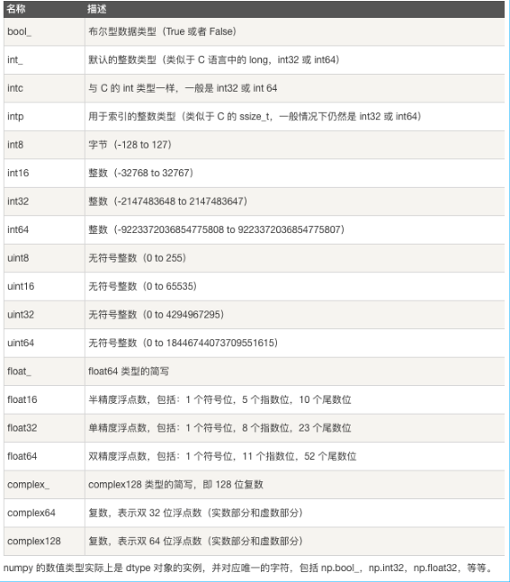

6. numpy indexing and slicing operations

Meaning: numpy array allows us to remove any specified local data

Index: a list of operations and empathy

arr[1]   # 取一行
arr[[1,2,3]]   # 取多行

slice:

1. Cut two lines before the data
```
arr[0:2]
```
2. The first two columns of data cut out
```
arr[:,0:2]
```
Reverse

1. column inversion
```
arr[:,::-1]
```
2. line inversion
```
arr[::-1]
```
3. Reverse the elements
```
arr[::-1,::-1]
```

Application: The downloaded picture reversal

# 查看图片的形状
img_arr.shape   # (554, 554, 3)

# 将一张图片反转
plt.imshow(img_arr[::-1,::-1,::-1])

7. Deformation reshape

Create an array

arr = np.array([[1,2,3],[4,5,6]])
arr.shape
print(arr)

# 结果：
array([[1, 2, 3],
       [4, 5, 6]])

The one-dimensional multi-dimensional change

arr_1 = arr.reshape((6,))
print(arr_1)

# 结果：
array([1, 2, 3, 4, 5, 6])

One-dimensional multi-dimensional change

arr_1.reshape((6,1))
# 结果：
array([[1],
       [2],
       [3],
       [4],
       [5],
       [6]])

arr_1.reshape((3,-1))   # -1表示自动计算行或者列数
# 结果：
array([[1, 2],
       [3, 4],
       [5, 6]])

8. cascade operation

Concept: numpy array is a plurality of horizontal or vertical mosaic, array dimensions must be consistent cascade

Define two arrays:

arr = array([[1, 2, 3],
              [4, 5, 6]])
n_arr = array([[1, 2, 3],
              [4, 5, 6]])
a = array([[1, 2],
       [3, 4]])

Match cascade: a shape of a plurality of cascaded arrays are exactly the same

import numpy as np

np.concatenate((arr,n_arr),axis=0)  # axis=0表示列，axis=1表示行

# 结果：
array([[1, 2, 3],
       [4, 5, 6],
       [1, 2, 3],
       [4, 5, 6]])

It does not match the cascade: the same dimensions, but inconsistent with the number of ranks

Horizontal cascade: the number of lines to ensure consistent

Longitudinal cascade: number of columns to ensure consistent

np.concatenate((a,arr),axis=1)

# 结果：
array([[1, 2, 1, 2, 3],
       [3, 4, 4, 5, 6]])

Application: The picture makes up nine squares

# 一行三张
arr_3 = np.concatenate((img_arr,img_arr,img_arr),axis=1)
# 三行九张
arr_9 = np.concatenate((arr_3,arr_3,arr_3),axis=0)
plt.imshow(arr_9)

9. broadcast mechanism

Definition: broadcast (Broadcast) is numpy different shapes (Shape) array of numerical embodiment, an array of arithmetic operations typically performed on the corresponding elements. If the two arrays a and b are the same shape, i.e., meet a.shape == b.shape, then the result is a * b a and b are multiplied by the corresponding bit array. This requires the same dimensions and the same length in each dimension.

Two identical shape array example:

Define two arrays:

x = array([[2, 2, 3],
            [1, 2, 3]])
y = array([[1, 1, 3],
          [2, 2, 4]])

For addition: x + y

# 结果：
array([[3, 3, 6],
       [3, 4, 7]])

Two different exemplary array shape:

Define two arrays:

arr1 = array([[0, 0, 0],
              [1, 1, 1],
              [2, 2, 2],
              [3, 3, 3]])
arr2 = array([1, 2, 3])

For adding: arr1 + arr2

# 结果：
array([[1, 2, 3],
       [2, 3, 4],
       [3, 4, 5],
       [4, 5, 6]])

Broadcast rules:
- All arrays are input to the array in which the shape of the longest par insufficient partial shape are preceded by a filled.
- Shape of the output array is the maximum value of each dimension of the input array shape.
- If the input of the same length and a dimension of the array corresponding to the array be calculated dimension, or length is 1, the array can be used to calculate, or error.
- When the length of the input array is a dimension 1, when calculating the dimension along a first set of values are used on this dimension.

10. The operation of conventional polymerization

Define an array:

arr = array([[1, 2, 3],
               [4, 5, 6]])

sum / sum

arr.sum(axis=1)
# 结果：array([ 6, 15])

max / maximum

arr.max(axis=1)
# 结果：array([ 3, 6])

min / Min

arr.min(axis=1)
# 结果：array([1, 4])

mean / average

arr.mean(axis=1)
# 结果：array([2., 5.])

11. The common mathematical functions

Commonly used mathematical functions:

1.NumPy provides standard trigonometric functions: sin (), cos (), tan ()

2.numpy.around (a, decimals) function returns the rounded value specified number.

Parameters: a: an array; decimals: rounding decimal places. The default value is 0. If negative, rounded to an integer of the decimal place of the left

Example:

arr = np.array([[1,2,3],[4,5,7]])

# 三角函数sin()：
np.sin(arr)
# 结果：
array([[ 0.84147098,  0.90929743,  0.14112001],
       [-0.7568025 , -0.95892427, -0.2794155 ]])

# 四舍五入：
arr = np.array([1.4,4.7,5.2])
np.around(arr,decimals=0)  # 对小数进行四舍五入
# 结果：
array([1., 5., 5.])

np.around(arr,decimals=-1)  # 对整数进行四舍五入
# 结果：
array([ 0.,  0., 10.])

12. The commonly used statistical functions

numpy.amin() 和 numpy.amax()，用于计算数组中的元素沿指定轴的最小、最大值。
numpy.ptp():计算数组中元素最大值与最小值的差（最大值 - 最小值）。
numpy.median() 函数用于计算数组 a 中元素的中位数（中值）
标准差std():标准差是一组数据平均值分散程度的一种度量。
- 公式：std = sqrt(mean((x - x.mean())**2))
- 如果数组是 [1，2，3，4]，则其平均值为 2.5。因此，差的平方是 [2.25,0.25,0.25,2.25]，并且其平均值的平方根除以 4，即 sqrt(5/4) ，结果为 1.1180339887498949。
方差var()：统计中的方差（样本方差）是每个样本值与全体样本值的平均数之差的平方值的平均数，即 mean((x - x.mean())** 2)。换句话说，标准差是方差的平方根。

示例：

# 定义一个数组：
arr = np.random.randint(60,100,size=(5,3))
array([[92, 75, 93],
       [85, 69, 97],
       [60, 78, 83],
       [63, 89, 76],
       [80, 78, 74]])

# 定轴最小值:numpy.amin()：
np.amin(arr,axis=1)
# 结果：
array([75, 69, 60, 63, 74])

# 定轴最大值与最小值差：numpy.ptp()
np.ptp(arr,axis=0)
# 结果：
array([32, 20, 23])

# 定轴中值：numpy.median()
np.median(arr,axis=0)
# 结果：
array([80., 78., 83.])

# 标准差：std = sqrt(mean((x - x.mean())**2))
arr = np.array([1,2,3,4,5])
# 方式一：
((arr - arr.mean())**2).mean()**0.5
# 方式二：
arr.std()

# 方差：mean((x - x.mean())**2)
arr.var()

13. 矩阵相关

矩阵：矩阵（Matrix）是一个按照长方阵列排列的复数或实数集合
单位矩阵：从左上角到右下角的对角线称为主对角线上的元素均为1。除此以外全都为0。
转置矩阵：将矩阵的行列互换得到的新矩阵称为转置矩阵，转置矩阵的行列式不变。

NumPy 中包含了一个矩阵库 numpy.matlib，该模块中的函数返回的是一个矩阵，而不是 ndarray 对象。一个的矩阵是一个由行（row）列（column）元素排列成的矩形阵列。

matlib.empty() 函数返回一个新的矩阵，语法格式为：numpy.matlib.empty(shape, dtype)，填充为随机数据

参数介绍：

shape: 定义新矩阵形状的整数或整数元组
Dtype: 可选，数据类型

示例:

import numpy.matlib as matlib
matlib.empty(shape=(5,6))

# 结果：
matrix([[1.16302223e-311, 1.16302228e-311, 1.16302223e-311,
         1.16302226e-311, 1.16302223e-311, 1.16302226e-311],
        [1.16302356e-311, 1.16302355e-311, 1.16302226e-311,
         1.16302222e-311, 1.16302222e-311, 1.16302226e-311],
        [1.16302223e-311, 1.16302223e-311, 1.16302747e-311,
         1.16302356e-311, 1.16302747e-311, 1.16302228e-311],
        [1.16302223e-311, 1.16302223e-311, 1.16302356e-311,
         1.16302449e-311, 1.16302228e-311, 1.16302228e-311],
        [1.16302364e-311, 1.16302364e-311, 1.16302226e-311,
         1.16302278e-311, 1.16302228e-311, 1.16302228e-311]])

numpy.matlib.zeros()，numpy.matlib.ones()返回填充为0或者1的矩阵

matlib.ones(shape=(3,4))

# 结果：
matrix([[1., 1., 1., 1.],
        [1., 1., 1., 1.],
        [1., 1., 1., 1.]])

numpy.matlib.eye() 函数返回一个矩阵，对角线元素为 1，其他位置为零。

numpy.matlib.eye(n, M,k, dtype)

参数说明：
- n: 返回矩阵的行数
- M: 返回矩阵的列数，默认为 n
- k: 对角线的索引
- dtype: 数据类型
示例：
```
matlib.eye(n=5,M=4,k=0)

# 结果：
matrix([[1., 0., 0., 0.],
        [0., 1., 0., 0.],
        [0., 0., 1., 0.],
        [0., 0., 0., 1.],
        [0., 0., 0., 0.]])
```

numpy.matlib.identity() 函数返回给定大小的单位矩阵。

单位矩阵是个方阵，从左上角到右下角的对角线（称为主对角线）上的元素均为 1，除此以外全都为 0。

示例：

matlib.identity(5)

# 结果：
matrix([[1., 0., 0., 0., 0.],
        [0., 1., 0., 0., 0.],
        [0., 0., 1., 0., 0.],
        [0., 0., 0., 1., 0.],
        [0., 0., 0., 0., 1.]])

转置矩阵：行转化列，列转化行

示例：

arr = np.random.randint(0,100,size=(5,5))
# 结果：
array([[51, 79, 17, 50, 53],
       [25, 48, 17, 32, 81],
       [80, 41, 90, 12, 30],
       [81, 17, 16,  0, 31],
       [73, 64, 38, 22, 96]])

arr.T
# 结果：
array([[51, 25, 80, 81, 73],
       [79, 48, 41, 17, 64],
       [17, 17, 90, 16, 38],
       [50, 32, 12,  0, 22],
       [53, 81, 30, 31, 96]])

矩阵相乘

numpy.dot(a, b, out=None)
- a : ndarray 数组
- b : ndarray 数组
矩阵乘以一个常数，就是所有位置都乘以这个数。

矩阵乘矩阵步骤：

第一个矩阵第一行的每个数字（2和1），各自乘以第二个矩阵第一列对应位置的数字（1和1），然后将乘积相加（ 2 x 1 + 1 x 1），得到结果矩阵左上角的那个值3。也就是说，结果矩阵第m行与第n列交叉位置的那个值，等于第一个矩阵第m行与第二个矩阵第n列，对应位置的每个值的乘积之和。