This article describes the use of pandas, summarizes some of the methods I use to machine learning process often.
# Pandas learning
Import pandas AS pd
 Import numpy AS NP
 Import Seaborn AS the SNS
 Import matplotlib.pyplot AS plt
 % matplotlib inline
 # Set pandas show all rows and columns, use better when more features
pd.set_option ( ' display.max_columns ' , None )
 # pd.set_option ( 'display.max_rows', None) # the general feeling is not required
1. Create data
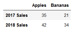
1.1 Creating a DataFrame , DataFrame data containers for the pandas, in fact, coupled with an array of column names, index names.
# 参数data,columns,index
# 方式1
fruit_sales = pd.DataFrame([[35, 21],[41,34]], columns=['Apples', 'Bananas'],index=['2017 Sales','2018 Sales'])
fruit_sales

# 方式2
fruit_sales2 = pd.DataFrame({'Apples':[35,42],'Bananas':[21,34]},index=['2017 Sales','2018 Sales'])
fruit_sales2
At least two ways the results are the same:
If you do not specify the index and columns, automatic digital assignment:

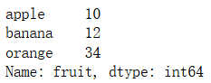
1.2, Series. DataFrame shows rows and columns, wherein each row or column is a Series.
# Series, represents only one data or a plurality of rows with DataFrame
items = [ ' Apple ' , ' Banana ' , ' Orange ' ]
the nums = [10,12,34 ]
fruit2 = pd.Series (the nums, = index items, = name ' Fruit ' )
fruit2
The results are:
2, the reader / csv file is stored, where the Titanic to kaggle training data item as an example.
train_data=pd.read_csv('train.csv',index_col=0)# 读取

train_data.to_csv('train_data.csv')# 存储
This method is common parameters are as follows:
filepath_or_buffer : file directory address
index_col : as to which column index
SkipRows : how many rows to skip at the beginning
skipfooter : how many rows to skip at the end
parse_dates : parsing date, there are a variety of input formats, with specific reference to the document. List suggestion input, such as [1,2,3], expressed 2,3,4 parsing date column
encoding : coding, such as Chinese and other available gbk, as reported coding error, please check this.
3, an overview of data and operations
3.1 The main method describe, info, head, columns, index, values, etc.
- head
train_data.head () # View the opening lines, default 5

- describe
train_data.describe () # display the description, only the default value of the column functions, you can include all the same as the second row, or column specifies a list
# train_data.describe (= the include 'All')
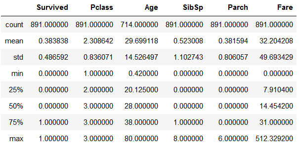
Or more, the number of statistics, maximum and minimum, mean, standard deviation, and a plurality of percentile values (specified percentage of the available list)
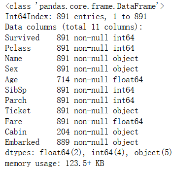
- info
train_data.info (verbose = True, null_counts = True) # Check the columns of data types, null values quantity
-
View shape, type, row, column
# 维度
train_data.shape
# size为shape 2个维度乘积
train_data.size

# DataFrame转np array
train_data.values# 即可

# 获取所有列名,行index
train_data.columns/index

# 查看所有数据类型
data.dtypes

# 一列或多列(多列时给个list)
ages=train_data.Age
ages=train_data['Age']

# 一行或多行
# 这2个相同
first_row=train_data.loc[0]
first_row=train_data.iloc[0]

# 多个行时不同
rows=train_data.iloc[1:3]# 第2,3行
rows=train_data.loc[1:3]# 第1,2,3行


# 同时筛选行和列。前面是选取的行,后面是选取的列
train_data.iloc[[1,2],[1,2]]
train_data.iloc[1:2,1:2]
3.2 复杂查询
#联合查询
a=train_data.loc[train_data.Pclass.isin([1,2]) & (train_data.Age<=30)]
#中位数
train_data.Age.median()
#平均值
train_data.Age.mean()
#查看该列包含种类(相当于set操作)
train_data.Pclass.unique()
#统计该列各个种类的数量(统计set后各元素出现的次数)
train_data.groupby('Pclass').size()# 结果按索引排序
train_data.Pclass.value_counts()# 这种方式更好,结果是按值排序的
#票价与年龄的比例,求比例最大的行号
idx=(train_data.Fare/train_data.Age).idxmax()
#查看此人是否存活
train_data.loc[idx,'Survived']
# 统计指定列为NaN的行数
train_data[train_data.Embarked.isna()]
# 统计指定列某条件下的行数
(train_data['Age']<50).sum()
# 统计所有Ticket中出现PC的次数
train_data.Ticket.map(lambda ticket:'PC' in ticket).sum()
3.3 数据操作
- DataFrame合并
# DataFrame合并
df1=pd.DataFrame(data={'price':[6,6.5,7],'count':[10,9,8]})
df2=pd.DataFrame(data={'name':['a','b'],'married':['Yes','Yes'],'price':[1,2]})
# 列名不同的添加列,相同列名的合并,数据按行合并
df=pd.concat([df1,df2],sort=False)

# 以2个df中指定列进行合并,合并的列名不必相同(此时第一列的列名为空),如果相同则作为index并将index排序
df1=pd.DataFrame(data={'price':[6,6.5,7],'count':[10,9,8],'sth':[2,3,4]})
df2=pd.DataFrame(data={'name':['yanfang','chenlun'],'married':['Yes','Yes'],'price':[1,10],'sth':[2,8]})

# 默认合并方式为left,即df1合并列(price,3)有多少行,结果就是多少行
# 除合并的列外,2个df不允许再出现同名的列
df=df1.set_index('price').join(df2.set_index('sth'),how='outer',sort=False)
# df=df1.set_index('price').join(df2.set_index('price'),how='outer',sort=False) 不允许重复列sth
- DataFrame属性修改
# 改变某列的数据类型,如将Age通过cut分段后,它的数据类型为categorical,而你想做PCA降维,那么只能转化为数值型
train_data['Age_bin']=train_data['Age_bin'].astype('float')
# 重命名列
data=data.rename(columns=dict(Pclass='Class',Fare='Ticket_price'))
# 重命名index
data=data.rename_axis("Id",axis=0)# 注意axis=1也可行,此时并未重命名index,而是将index作为一列,给予它一个列名
- groupby 分类(查询)
# groupby分类
df=pd.DataFrame(data=[[20,7],[10,11],[10,8],[20,12],[9,8]],columns=['price','points'])
# 输出各价钱对应的最高分数
df.groupby('price')['points'].max().sort_index(axis=0)#对于Series,它只有一列数据,axis必须为0
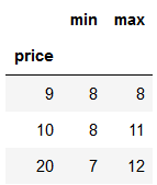
# agg:以多个函数操作的结果作为各个列 both=df.groupby('price').points.agg([min,max]) both
- 联合排序
# 多个列的排序
data=train_data.iloc[:10,4:6]
data.sort_values(by=['Age','SibSp'])

- 数据修改
# map修改数据,apply是另一个修改方法
train_datan['Ticket']=train_data.Ticket.map(lambda ticket:'PC' in ticket)# 变为布尔类型

# 增加列:将Age按年龄段分类,此时该列的数据类型为categorical
train_data['Age_bin']=pd.cut(train_data['Age'],bins=[0,25,40,55,95],labels=[1,2,3,4])
# get_dummies对类别型的列做one-hot处理,之后我们就可以如下查看相关系数了
data_show=pd.get_dummies(train_data,columns=['Age_bin'])
sns.heatmap(data_show.corr(),annot=True,cmap='RdYlGn',linewidths=0.2)

# 缺失值处理:之前的map,apply,以及此处的fillna,replace等都可以修改数据。
# 以中位数填充None/NaN值
train_data.Age.fillna(train_data.Age.median(),inplace=True)
# 如果该列缺少太多数据,可直接原地(inplace)删除该列
train_data.drop(['Age'],axis=1,inplace=True)
# 使用replace替换属性中的值
train_data.Age.replace(28,30)
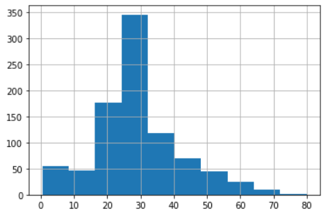
4 可视化
df可以直接用matplotlib可视化
train_data['Age'].hist()# 统计各个年龄的数量,作直方图