Reference: "Machine Learning"
principle
sample n-dimensional Gaussian distribution is:
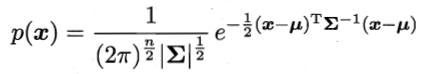
Σ is the covariance matrix
By the Bayes' theorem, the sample belonging to class i Xj posterior probability is:
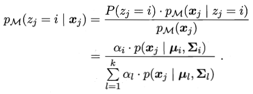
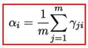
The abbreviated formula for the gamma] JI
The formula for the sample Xj Category

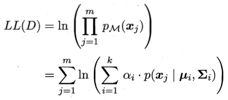
Each classification to a coefficient, using the log-likelihood, have
Derivative of the above formula were Σ, μ, so the derivative is 0, to give


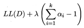
Summing coefficient is 1, this constraint is introduced, in the form of log likelihood Lagrangian is
The coefficient α of the derivative of formula, so the derivative is 0, to give
Above, red frame part is the parameter update formula, particularly relates to a derivative of the scalar vector / matrix derivation, generally Differentiation Method, your own Now derivation rules.
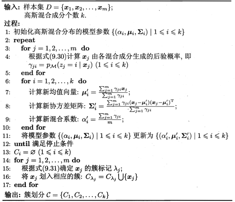
Algorithmic process is:
Implementation code:
data set
4.0 watermelon data set using, as follows
序号,密度,含糖量
1,0.697,0.460
2,0.774,0.376
3,0.634,0.264
4,0.608,0.318
5,0.556,0.215
6,0.403,0.237
7,0.481,0.149
8,0.437,0.211
9,0.666,0.091
10,0.243,0.267
11,0.245,0.057
12,0.343,0.099
13,0.639,0.161
14,0.657,0.198
15,0.360,0.370
16,0.593,0.042
17,0.719,0.103
18,0.359,0.188
19,0.339,0.241
20,0.282,0.257
21,0.748,0.232
22,0.714,0.346
23,0.483,0.312
24,0.478,0.437
25,0.525,0.369
26,0.751,0.489
27,0.532,0.472
28,0.473,0.376
29,0.725,0.445
30,0.446,0.459
代码
# 1 读取数据
file='xigua4.txt'
x=[]
with open(file) as f:
    f.readline()
    lines=f.read().split('\n')
    for line in lines:
        data=line.split(',')
        x.append([float(data[-2]),float(data[-1])])
y=np.array(x)
# 2 算法部分
import numpy as np
import random

def probability(x,u,cov):
    cov_inv=np.linalg.inv(cov)
    cov_det=np.linalg.det(cov)
    return np.exp(-1/2*((x-u).T.dot(cov_inv.dot(x-u))))/np.sqrt(cov_det)


def gauss_mixed_clustering(x,k=3,epochs=50,reload_params=None):
    features_num=len(x[0])
    r=np.empty(shape=(len(x),k))
#     初始化系数,均值向量和协方差矩阵
    if reload_params!=None:
        a,u,cov=reload_params
    else:
        a=np.random.uniform(size=k)
        a/=np.sum(a)
        u=np.array(random.sample(list(x),k))
        cov=np.empty(shape=(k,features_num,features_num))
#         初始化为只有对角线不为0
        for i in range(k):
            for j in range(features_num):
                cov[i][j]=[0]*j+[0.5]+[0]*(features_num-j-1)
    step=0
    while step<epochs:
#         E步:计算r_ji
        for j in range(len(x)):
            for i in range(k):
                r[j,i]=a[i]*probability(x[j],u[i],cov[i])
            r[j]/=np.sum(r[j])

        for i in range(k):
            r_toal=np.sum(r[:,i])
            u[i]=np.sum([x[j]*r[j,i] for j in range(len(x))],axis=0)/r_toal
            cov[i]=np.sum([r[j,i]*((x[j]-u[i]).reshape((features_num,1)).dot((x[j]-u[i]).reshape((1,features_num)))) for j in range(len(x))],axis=0)/r_toal
            a[i]=r_toal/len(x)
        step+=1
    C=[]
    for i in range(k):
        C.append([])
    for j in range(len(x)):
        c_j=np.argmax(r[j,:])
        C[c_j].append(x[j])
    return C,a,u,cov
验证
res,A,U,COV=gauss_mixed_clustering(y)
import matplotlib.pyplot as plt
%matplotlib inline
colors=['green','blue','red','black','yellow','orange']
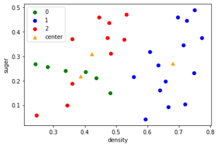
for i in range(len(res)):
plt.scatter([d[0] for d in res[i]],[d[1] for d in res[i]],color=colors[i],label=str(i))
plt.scatter([d[0] for d in U],[d[1] for d in U],color=colors[-1],marker='^',label='center')
plt.xlabel('density')
plt.ylabel('suger')
plt.legend()
50轮后

# 100轮
res,A,U,COV=gauss_mixed_clustering(y,reload_params=[A,U,COV])
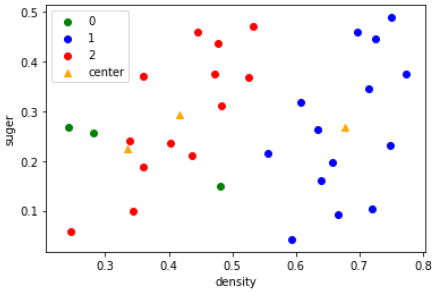
for i in range(len(res)):
plt.scatter([d[0] for d in res[i]],[d[1] for d in res[i]],color=colors[i],label=str(i))
plt.scatter([d[0] for d in U],[d[1] for d in U],color=colors[-1],marker='^',label='center')
plt.xlabel('density')
plt.ylabel('suger')
plt.legend()
# 200轮后不再变化
res,A,U,COV=gauss_mixed_clustering(y,epochs=100,reload_params=[A,U,COV])
for i in range(len(res)):
    plt.scatter([d[0] for d in res[i]],[d[1] for d in res[i]],color=colors[i],label=str(i))
plt.scatter([d[0] for d in U],[d[1] for d in U],color=colors[-1],marker='^',label='center')
plt.xlabel('density')
plt.ylabel('suger')
plt.legend()
总结
这个算法本身不复杂,可能涉及到矩阵求导的部分会麻烦一点。西瓜数据集太小了,收敛非常快。然后,这个算法同样对于初值敏感。