This article describes how to use Gaussian mixture models to split a one-dimensional multimodal distribution into multiple distributions.

Gaussian Mixture Models (GMM) is a probabilistic model commonly used in the fields of statistics and machine learning for modeling and analyzing complex data distributions. GMM is a generative model that assumes that the observed data is composed of multiple Gaussian distributions, each Gaussian distribution is called a component, and these components are weighted to control their contribution in the data.
Generate data with multimodal distributions
It often occurs when a data set exhibits multiple distinct peaks or modes, each representing a prominent cluster or concentration of data points in the distribution. These patterns can be thought of as high-density areas where data values are more likely to occur.
We will use a 1D array generated by numpy.
 import numpy as np

 dist_1 = np.random.normal(10, 3, 1000)
 dist_2 = np.random.normal(30, 5, 4000)
 dist_3 = np.random.normal(45, 6, 500)

 multimodal_dist = np.concatenate((dist_1, dist_2, dist_3), axis=0)
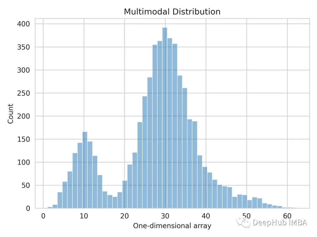
Let's visualize a one-dimensional data distribution.
 import matplotlib.pyplot as plt
 import seaborn as sns
 sns.set_style('whitegrid')

 plt.hist(multimodal_dist, bins=50, alpha=0.5)
 plt.show()
Split multimodal distributions using Gaussian mixture models
Below we will separate the multimodal distributions back into the three original distributions by using a Gaussian mixture model to calculate the mean and standard deviation of each distribution. The Gaussian mixture model is a probabilistic unsupervised model that can be used for data clustering. It estimates the density area using the expectation maximization algorithm.
 from sklearn.mixture import GaussianMixture

 gmm = GaussianMixture(n_components=3)
 gmm.fit(multimodal_dist.reshape(-1, 1))

 means = gmm.means_

 # Conver covariance into Standard Deviation
 standard_deviations = gmm.covariances_**0.5

 # Useful when plotting the distributions later
 weights = gmm.weights_


 print(f"Means: {means}, Standard Deviations: {standard_deviations}")

 #Means: [29.4, 10.0, 38.9], Standard Deviations: [4.6, 3.1, 7.9]
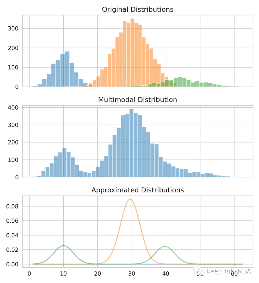
Now that we have the mean and standard deviation, we can model the original distribution. You can see that while the mean and standard deviation may not be exactly correct, they provide a close estimate.
Compare our estimates with the original data.
 from scipy.stats import norm

 fig, axes = plt.subplots(nrows=3, ncols=1, sharex='col', figsize=(6.4, 7))

 for bins, dist in zip([14, 34, 26], [dist_1, dist_2, dist_3]):
     axes[0].hist(dist, bins=bins, alpha=0.5)

 axes[1].hist(multimodal_dist, bins=50, alpha=0.5)

 x = np.linspace(min(multimodal_dist), max(multimodal_dist), 100)

 for mean, covariance, weight in zip(means, standard_deviations, weights):
     pdf = weight*norm.pdf(x, mean, std)
     plt.plot(x.reshape(-1, 1), pdf.reshape(-1, 1), alpha=0.5)

 plt.show()
Summarize
The Gaussian mixture model is a powerful tool that can be used to model and analyze complex data distributions. It is also one of the foundations of many machine learning algorithms. Its application scope covers many fields and can solve various data modeling and analysis problems.
This approach can be used as a feature engineering technique to estimate confidence intervals for subdistributions within input variables.
https://avoid.overfit.cn/post/2d68eddf58c04732a4826c6d6c2d1a50
Author: Adrian Evensen