Depth study into the pit of the five notes --- analyze fuel efficiency

Disclaimer: This article is a blogger original article, follow the CC 4.0 BY-SA copyright agreement, reproduced, please attach the original source link and this statement.

This link: https://blog.csdn.net/LEEANG121/article/details/102510944

The official note from Tensorflow tutorial Basic regression: Predict fuel efficiency. The main content of the data for some brief description.
Original tutorial uses the classic AUTO MPG data set was constructed in the late 1970s and early 1980s automobile fuel efficiency of the model to predict. Model is predicted target fuel efficiency-MPG, the parameters comprising: number of cylinders, displacement, horsepower and weight and the like.

Fuel efficiency data sets acquired

#搭建环境，引入数据库
from __future__ import absolute_import, division, print_function, unicode_literals
import warnings
warnings.filterwarnings('ignore')
import pathlib

import matplotlib.pyplot as plt
import pandas as pd
import seaborn as sns

import tensorflow as tf

from tensorflow import keras
from tensorflow.keras import layers

The first step, first download the data set

dataset_path = keras.utils.get_file("auto-mpg.data", "http://archive.ics.uci.edu/ml/machine-learning-databases/auto-mpg/auto-mpg.data")
dataset_path

'C:\\Users\\DELL\\.keras\\datasets\\auto-mpg.data'

Since I downloaded the data set before, thus directly displays the storage location of the data set, before importing the data set with pandas, we can open our first downloadable data sets with VS, take a look at what specific data set

as shown above I intercepted the last few lines of the data set, the last few lines of the reasons for the interception will be explained below. Now we import label data set column with pandas

column_names = ['MPG', 'Cylinders','Displacement','Horsepower','Weight',
                'Acceleration', 'Model Year', 'Origin']#添加列标签
#读取csv文件，其中第一行引入列标签
raw_dataset = pd.read_csv(dataset_path, names=column_names,
                      na_values = "?", comment='\t',
                      sep=" ", skipinitialspace=True)
dataset = raw_dataset.copy()
dataset.tail()#显示最后五行数据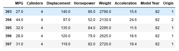                     

The figure shows that the data set last five lines of data, which is why we shot the last few rows of ~

Cleaning data

Dataset contains some erroneous data, we need to detect and clear out

dataset.isna().sum()#ISNA函数，是用来检测一个值是否为#N/A，返回TRUE或FALSE

In the above code, the ISNA function, is used to detect whether a value # N / A, returns TRUE or FALSE

MPG             0
Cylinders       0
Displacement    0
Horsepower      6
Weight          0
Acceleration    0
Model Year      0
Origin          0
dtype: int64

In order to ensure simplicity of this initial example, delete those lines.

dataset = dataset.dropna()

Where, 'Origin' column represents the actual classification, rather than a number. Therefore, it is converted to hot code (one-hot)

origin = dataset.pop('Origin')#删除最后一列的数据，同时返回该列元素的数值
#把最后一列分别换成USA Europe 和 Japan
dataset['USA'] = (origin == 1)*1.0
dataset['Europe'] = (origin == 2)*1.0
dataset['Japan'] = (origin == 3)*1.0
dataset.tail()#显示最后五行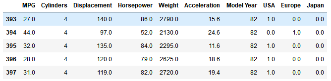

Split the training data set and test data set

Since the original data set does not elaborate divided into training and test sets, so we need to re-set the dismantling of the original data set and the training data set
precision model training for the training set, with the test set to test the model.

train_dataset = dataset.sample(frac=0.8,random_state=0)
test_dataset = dataset.drop(train_dataset.index)

Separation eigenvalues

Separated from the target feature values ​​or 'tags' so that the tag data and parameter data are separated, the training is a prerequisite. This tag is also training model predicted values.

train_labels = train_dataset.pop('MPG')#删除训练集‘MPG’标签，并返回相应的值
test_labels = test_dataset.pop('MPG')#删除测试集‘MPG’标签，并返回相应的值

Data normalization

def norm(x):
   return (x - train_stats['mean']) / train_stats['std']
normed_train_data = norm(train_dataset)
normed_test_data = norm(test_dataset)

Note that the statistics (mean and standard deviation) of the normalized output needs to be fed back to the model, which apply to any other data, as well as hot code we obtained before.

model

Modeling the way as the previous articles, followed by building a model - that is to build neural network model to build the network layer through the training model and predict and evaluate models. All codes are from the official tutorial. Here are the code only, not specifically explained.

def build_model():
  model = keras.Sequential([
    layers.Dense(64, activation='relu', input_shape=[len(train_dataset.keys())]),
    layers.Dense(64, activation='relu'),
    layers.Dense(1)
  ])
  optimizer = tf.keras.optimizers.RMSprop(0.001)
  model.compile(loss='mse',optimizer=optimizer, metrics=['mae', 'mse'])
  return model
  model = build_model

After the model is built, we examine the overall structure

model.summary()

Model: "sequential"
_________________________________________________________________
Layer (type)                 Output Shape              Param #   
=================================================================
dense (Dense)                (None, 64)                640       
_________________________________________________________________
dense_1 (Dense)              (None, 64)                4160      
_________________________________________________________________
dense_2 (Dense)              (None, 1)                 65        
=================================================================
Total params: 4,865
Trainable params: 4,865
Non-trainable params: 0

Trainer

The model training for 1,000 cycles, and record the training and validation of accuracy.

# 通过为每个完成的时期打印一个点来显示训练进度
class PrintDot(keras.callbacks.Callback):
  def on_epoch_end(self, epoch, logs):
    if epoch % 100 == 0: print('')
    print('.', end='')

EPOCHS = 1000
history = model.fit(
   normed_train_data, train_labels,
   epochs=EPOCHS, validation_split = 0.2, verbose=0,
   callbacks=[PrintDot()])

....................................................................................................
....................................................................................................
....................................................................................................
....................................................................................................
....................................................................................................
....................................................................................................
....................................................................................................
....................................................................................................
....................................................................................................
....................................................................................................    

Use history stored in the object of statistical information visualization training schedule model.

hist = pd.DataFrame(history.history)
hist['epoch'] = history.epoch
hist.tail()#显示最后五条训练信息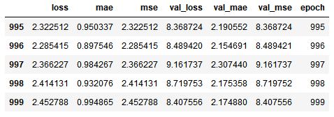

Next, a graph with changes in the error iterations performed by graphically

def plot_history(history):
   hist = pd.DataFrame(history.history)
   hist['epoch'] = history.epoch
   
   plt.figure()
   plt.xlabel('Epoch')
   plt.ylabel('Mean Abs Error [MPG]')
   plt.plot(hist['epoch'], hist['mae'],
           label='Train Error')
   plt.plot(hist['epoch'], hist['val_mae'],
           label = 'Val Error')
   plt.ylim([0,5]
   plt.legend()
   plt.figure()
   plt.xlabel('Epoch')
   plt.ylabel('Mean Square Error [$MPG^2$]')
   plt.plot(hist['epoch'], hist['mse'],
           label='Train Error')
   plt.plot(hist['epoch'], hist['val_mse'],
           label = 'Val Error')
   plt.ylim([0,20])
   plt.legend()
   plt.show()
plot_history(history)

From the chart found, verify the value after 100 cycles, we began to deteriorate, and now we adjusted model.fit, training again. We will use a EarlyStopping callback to test the training conditions of each epoch. If there is no improvement after a certain number of epochs, the automatic stop training.

model = build_model()
# patience 值用来检查改进 epochs 的数量
early_stop = keras.callbacks.EarlyStopping(monitor='val_loss', patience=10)
history = model.fit(normed_train_data, train_labels, epochs=EPOCHS,
                    validation_split = 0.2, verbose=0, callbacks=[early_stop, PrintDot()])

plot_history(history)

prediction

Now use the test set of data to predict

test_predictions = model.predict(normed_test_data).flatten()
plt.scatter(test_labels, test_predictions)
plt.xlabel('True Values [MPG]')
plt.ylabel('Predictions [MPG]')
plt.axis('equal')
plt.axis('square')
plt.xlim([0,plt.xlim()[1]])
plt.ylim([0,plt.ylim()[1]])
_ = plt.plot([-100, 100], [-100, 100])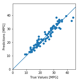

in conclusion

Mean square error (MSE) is a common problem return for the loss of function (classification using different loss function).
Similarly, the evaluation index for regression and classification different. Common Regression indicator is the average absolute error (MAE).
When there is a range of different characteristics of the digital input data, each feature independently be scaled to the same range.
If the training data is small, a method of selecting fewer small network hidden layer to avoid overfitting.
Early stops is an effective technique to prevent over-fitting.