Scatter line graph plotted Python_

In the process of data analysis, it is often necessary to visualize the data currently commonly used: line graph scattergram  

Import the necessary external package is a drawing to import a font

import matplotlib.pyplot as plt
from matplotlib.font_manager import FontProperties

We need to get the data before data processing to obtain the required data from TXT XML csv excel and other text, save to list

 1 def GetFeatureList(full_path_file):
 2     file_name = full_path_file.split('\\')[-1][0:4]
 3     # print(file_name)
 4     # print(full_name)
 5     K0_list = []
 6     Area_list = []
 7     all_lines = []
 8     f = open(full_path_file,'r')
 9     all_lines = f.readlines()
10     lines_num = len(all_lines)
11     # 数据清洗
12     if lines_num > 5000:
13         for i in range(3,lines_num-1):
14             temp_k0 = int(all_lines[i].split('\t')[1])
15             if temp_k0 == 0:
16                 K0_list.append(ComputK0(all_lines[i]))
17             else:
18                 K0_list.append(temp_k0)
19             Area_list.append(float(all_lines[i].split('\t')[15]))
20         # K0_Scatter(K0_list,Area_list,file_name)
21     else:
 22 is          Print ( ' {} The sample amount is less than 5000 ' .format (file_name))
 23 is      return K0_list, Area_list, file_name

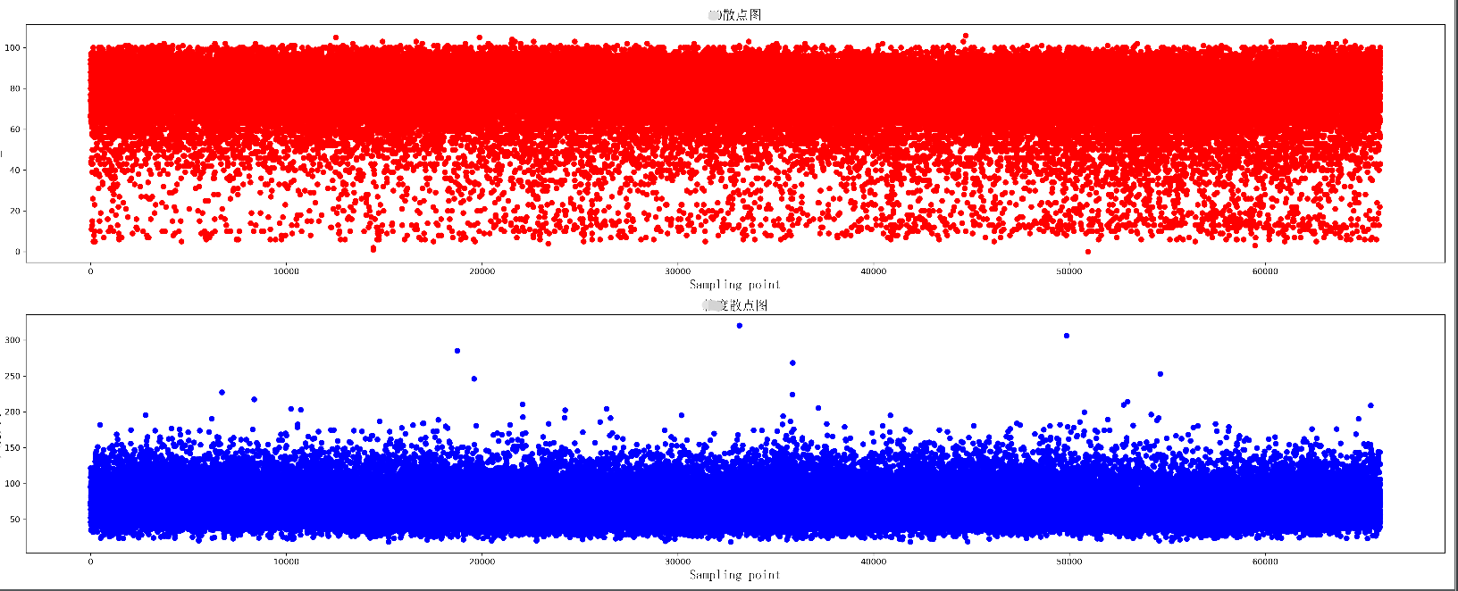
Draw a scatter plot two sets of data, while drawing two scatter plots, distributed up and down in the same picture

. 1  DEF K0_Scatter (K0_list, area_list, pic_name):
 2      plt.figure (figsize = (25, 10), = 300 dpi )
 . 3      # imported Chinese font, and font size 
. 4      zhfont = FontProperties (fname = ' C: / the Windows / Fonts / the simsun.ttc ' , size = 16 )
 . 5      AX = plt.subplot (211 )
 . 6      # Print (K0_list) 
. 7      ax.scatter (Range (len (K0_list)), K0_list, C = ' R & lt ' , = marker ' O ' )
 . 8      plt.title (U ' scattergram ' , fontproperties = zhfont)
 9     plt.xlabel('Sampling point', fontproperties=zhfont)
11     plt.ylabel('K0_value', fontproperties=zhfont)
12     ax = plt.subplot(212)
13     ax.scatter(range(len(area_list)), area_list, c='b', marker='o')
14     plt.xlabel('Sampling point', fontproperties=zhfont)
15     plt.ylabel(u'大小', fontproperties=zhfont)
16     plt.title(u'散点图', fontproperties=zhfont)
17     # imgname = 'E:\\' + pic_name + '.png'
18     # plt.savefig(imgname, bbox_inches = 'tight')
19     plt.show()

Scatter display

 

 

 Draw a line chart of data increases for each tag

. 1  DEF K0_Plot (in X_LABEL, Y_LABEL, pic_name):
 2      plt.figure (figsize = (25, 10), = 300 dpi )
 . 3      # imported Chinese font, and font size 
. 4      zhfont = FontProperties (fname = ' C: / the Windows / Fonts / the simsun.ttc ' , size = 16 )
 . 5      AX = plt.subplot (111 )
 . 6      # Print (K0_list) 
. 7      ax.plot (in X_LABEL, Y_LABEL, C = ' R & lt ' , marker = ' O ' )
 . 8      PLT. title (pic_name, fontproperties = zhfont)
 . 9      plt.xlabel ( 'coal_name', fontproperties=zhfont)
10     plt.ylabel(pic_name, fontproperties=zhfont)
11     # ax.xaxis.grid(True, which='major')
12     ax.yaxis.grid(True, which='major')
13     for a, b in zip(X_label, Y_label):
14         str_label = a + str(b) + '%'
15         plt.text(a, b, str_label, ha='center', va='bottom', fontsize=10)
16     imgname = 'E:\\' + pic_name + '.png'
17     plt.savefig(imgname, bbox_inches = 'tight')
18     # plt.show()

 

 Drawing a plurality of line graphs

. 1  DEF K0_MultPlot (dis_name, dis_lsit, pic_name):
 2      plt.figure (figsize = (80, 10), = 300 dpi )
 . 3      # imported Chinese font, and font size 
. 4      zhfont = FontProperties (fname = ' C: / the Windows / Fonts / the simsun.ttc ' , size = 16 )
 . 5      AX = plt.subplot (111 )
 . 6      in X_LABEL Range = (len (dis_lsit [. 1 ]))
 . 7      P1 = ax.plot (in X_LABEL, dis_lsit [. 1], C = ' R & lt ' , marker = ' O ' , label = ' the Euclidean Distance ' )
 . 8     p2 = ax.plot(X_label, dis_lsit[2], c='b', marker='o',label='Manhattan Distance')
 9     p3 = ax.plot(X_label, dis_lsit[4], c='y', marker='o',label='Chebyshev Distance')
10     p4 = ax.plot(X_label, dis_lsit[5], c='g', marker='o',label='weighted Minkowski Distance')
11     plt.legend()
12     plt.title(pic_name, fontproperties=zhfont)
13     plt.xlabel('coal_name', fontproperties=zhfont)
14     plt.ylabel(pic_name, fontproperties=zhfont)
15     # ax.xaxis.grid(True, which='major')
16     ax.yaxis.grid(True, which='major')
17     for a, b,c in zip(X_label, dis_lsit[5],dis_name):
18         str_label = c + '_'+ str(b)
19         plt.text(a, b, str_label, ha='center', va='bottom', fontsize=5)
20     imgname = 'E:\\' + pic_name + '.png'
21     plt.savefig(imgname,bbox_inches = 'tight')
22     # plt.show()

 

 There are many tips graphic display, so that a better visualization, such as custom axis scale, grid, etc., a subsequent finishing