A task
This time we will learn the use of support vector machine and adjust some parameters in machine learning. Support vector machine is a basic principle of the low-dimensional problem can not be separated into high-dimensional separable problem, in front of the blog specifically introduced, there is no longer introduced.
First import the relevant standard library:
matplotlib inline%
Import numpy AS NP
Import matplotlib.pyplot AS PLT
from stats SciPy Import

Import Seaborn AS SNS; sns.set () # Seaborn using default settings
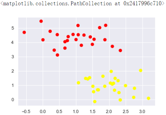
As an example, we first generate some random data, taking into account the simple task of classification, which is a good point two categories separated:
# Random point data to generate data sets for clustering make_blobs
from sklearn.datasets.samples_generator Import make_blobs

# Center: generating center point data, the default value. 3
X-, Y = make_blobs (N_SAMPLES = 50, 2 = Centers, random_state = 0, = 0.60 cluster_std)
plt.scatter (X-[:, 0], X-[:,. 1], Y = C, S = 50, = CMap 'Autumn')
Draw a scatter plot of the data for the current distribution
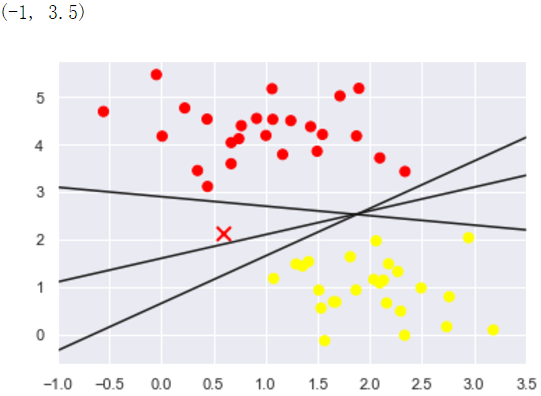
We will try to draw a line separating the two sets of data to create a classification model. For the two-dimensional data shown here, which we can complete the task manually. But once we see a problem: there are more than two possible dividing line can be divided into two categories perfect area!
xfit = np.linspace(-1, 3.5)
plt.scatter(X[:, 0], X[:, 1], c=y, s=50, cmap='autumn')
plt.plot([0.6], [2.1], 'x', color='red', markeredgewidth=2, markersize=10)

for m, b in [(1, 0.65), (0.5, 1.6), (-0.2, 2.9)]:
    plt.plot(xfit, m * xfit + b, '-k')

plt.xlim(-1, 3.5)
These are separated by three different lines, however, these can be separated completely straight distinguish these samples. Clearly, our simple intuition, "between classification dash" is not enough, we need to reflect further on, according to ideological support vector machine, so the effect is not ideal division.
SVM provides an improved method. Intuition is this: We are not among the classification, simply draw a straight line of zero width, but the margin is certain to draw a straight line width, until recently the point. This is an example:
xfit = np.linspace(-1, 3.5)
plt.scatter(X[:, 0], X[:, 1], c=y, s=50, cmap='autumn')

for m, b, d in [(1, 0.65, 0.33), (0.5, 1.6, 0.55), (-0.2, 2.9, 0.2)]:
    yfit = m * xfit + b
    plt.plot(xfit, yfit, '-k')
    plt.fill_between(xfit, yfit - d, yfit + d, edgecolor='none',
                     color='#AAAAAA', alpha=0.4) # alpha透明度

plt.xlim(-1, 3.5);
如图所示
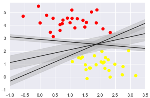
在支持向量机中,边距最大化的直线是我们将选择的最优模型。 支持向量机是这种最大边距估计器的一个例子。
二、训练一个基本的SVM
我们来看看这个数据的实际结果:我们将使用 sklearn 的支持向量分类器,对这些数据训练 SVM 模型。 目前,我们将使用一个线性核并将C参数设置为一个默认的数值。
from sklearn.svm import SVC  # Support Vector Classifier
model = SVC(kernel='linear') # 线性核函数
model.fit(X, y)
得到的SVM模型为
SVC(C=1.0, cache_size=200, class_weight=None, coef0=0.0,
    decision_function_shape='ovr', degree=3, gamma='auto_deprecated',
    kernel='linear', max_iter=-1, probability=False, random_state=None,
    shrinking=True, tol=0.001, verbose=False)
为了更好展现这里发生的事情,让我们创建一个辅助函数,为我们绘制 SVM 的决策边界。
#绘图函数
def plot_svc_decision_function(model, ax=None, plot_support=True):
    """Plot the decision function for a 2D SVC"""
    if ax is None:
        ax = plt.gca() # get子图
    xlim = ax.get_xlim()
    ylim = ax.get_ylim()

    # create grid to evaluate model
    x = np.linspace(xlim[0], xlim[1], 30)
    y = np.linspace(ylim[0], ylim[1], 30)
    Y, X = np.meshgrid(y, x) # 生成网格点和坐标矩阵
    xy = np.vstack([X.ravel(), Y.ravel()]).T     # 堆叠数组
    P = model.decision_function(xy).reshape(X.shape)

    # plot decision boundary and margins
    ax.contour(X, Y, P, colors='k',
               levels=[-1, 0, 1], alpha=0.5,
               linestyles=['--', '-', '--']) # 生成等高线 - -

    # plot support vectors
    if plot_support:
        ax.scatter(model.support_vectors_[:, 0],
                   model.support_vectors_[:, 1],
                   s=300, linewidth=1, facecolors='none');
    ax.set_xlim(xlim)
    ax.set_ylim(ylim)
绘出决策边界
plt.scatter(X[:, 0], X[:, 1], c=y, s=50, cmap='autumn')
plot_svc_decision_function(model);
如图所示:
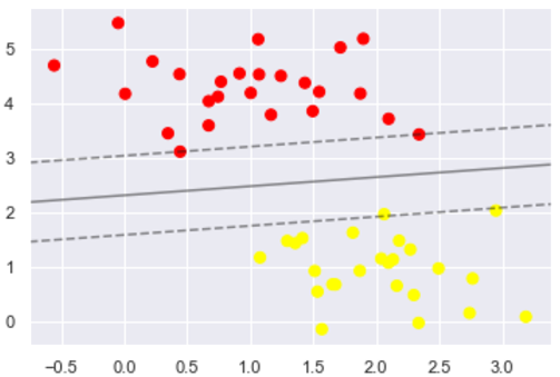
这是最大化两组点之间的间距的分界线,那中间这条线就是我们最终的决策边界了。 请注意,一些训练点碰到了边缘, 这些点是这种拟合的关键要素,被称为支持向量。 在 Scikit-Learn 中,这些点存储在分类器的support_vectors_属性中:
model.support_vectors_
得到的支持向量的结果
array([[0.44359863, 3.11530945],
       [2.33812285, 3.43116792],
       [2.06156753, 1.96918596]])
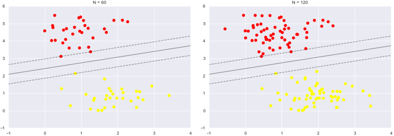
在支持向量机只有位于支持向量上面的点才会对决策边界有影响,也就是说不管有多少的点是非支持向量,那对最终的决策边界都不会产生任何影响。我们可以看到这一点,例如,如果我们绘制该数据集的前 60 个点和前120个点获得的模型:
def plot_svm(N=10, ax=None):
    X, y = make_blobs(n_samples=200, centers=2,
                      random_state=0, cluster_std=0.60)
    X = X[:N]
    y = y[:N]
    model = SVC(kernel='linear', C=1E10)
    model.fit(X, y)

    ax = ax or plt.gca()
    ax.scatter(X[:, 0], X[:, 1], c=y, s=50, cmap='autumn')
    ax.set_xlim(-1, 4)
    ax.set_ylim(-1, 6)
    plot_svc_decision_function(model, ax)

fig, ax = plt.subplots(1, 2, figsize=(16, 6))
fig.subplots_adjust(left=0.0625, right=0.95, wspace=0.1)
for axi, N in zip(ax, [60, 120]):
    plot_svm(N, axi)
    axi.set_title('N = {0}'.format(N))
观察可以发现分别使用60个和120个数据点,决策边界却没有发生变化。所有只要支持向量没变,其他的数据怎么加无所谓!
三、引入核函数的SVM
首先我们先用线性的核来看一下在下面这样比较难的数据集上还能分了吗?
from sklearn.datasets.samples_generator import make_circles
X, y = make_circles(100, factor=.1, noise=.1) # 二维圆形数据 factor 内外圆比例 (0,1)

clf = SVC(kernel='linear').fit(X, y)

plt.scatter(X[:, 0], X[:, 1], c=y, s=50, cmap='autumn')
plot_svc_decision_function(clf, plot_support=False);
数据集如图所示:
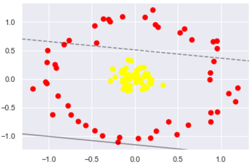
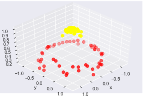
很明显,用线性分类分不了了,那咋办呢?试试高维核变换吧!
#加入了新的维度r
from mpl_toolkits import mplot3d
r = np.exp(-(X ** 2).sum(1))
def plot_3D(elev=30, azim=30, X=X, y=y):
    ax = plt.subplot(projection='3d')
    ax.scatter3D(X[:, 0], X[:, 1], r, c=y, s=50, cmap='autumn')
    ax.view_init(elev=elev, azim=azim) # 设置3D视图的角度  一般都为45
    ax.set_xlabel('x')
    ax.set_ylabel('y')
    ax.set_zlabel('r')

plot_3D(elev=45, azim=45, X=X, y=y)
画出刚才的数据集的一个3维图像
在 Scikit-Learn 中,我们可以通过使用kernel模型超参数,将线性核更改为 RBF(径向基函数,也叫高斯核函数)核来进行核变换,先暂时不管C参数:
#加入径向基函数
clf = SVC(kernel='rbf', C=1E6)
clf.fit(X, y)
得到的SVM模型为
SVC(C=1000000.0, cache_size=200, class_weight=None, coef0=0.0,
    decision_function_shape='ovr', degree=3, gamma='auto_deprecated',
    kernel='rbf', max_iter=-1, probability=False, random_state=None,
    shrinking=True, tol=0.001, verbose=False)
再次进行分类任务
#这回牛逼了!
plt.scatter(X[:, 0], X[:, 1], c=y, s=50, cmap='autumn')
plot_svc_decision_function(clf)
plt.scatter(clf.support_vectors_[:, 0], clf.support_vectors_[:, 1],
            s=300, lw=1, facecolors='none');
分类结果如图
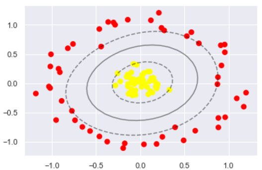
使用这种核支持向量机,我们学习一个合适的非线性决策边界。这种核变换策略在机器学习中经常被使用!
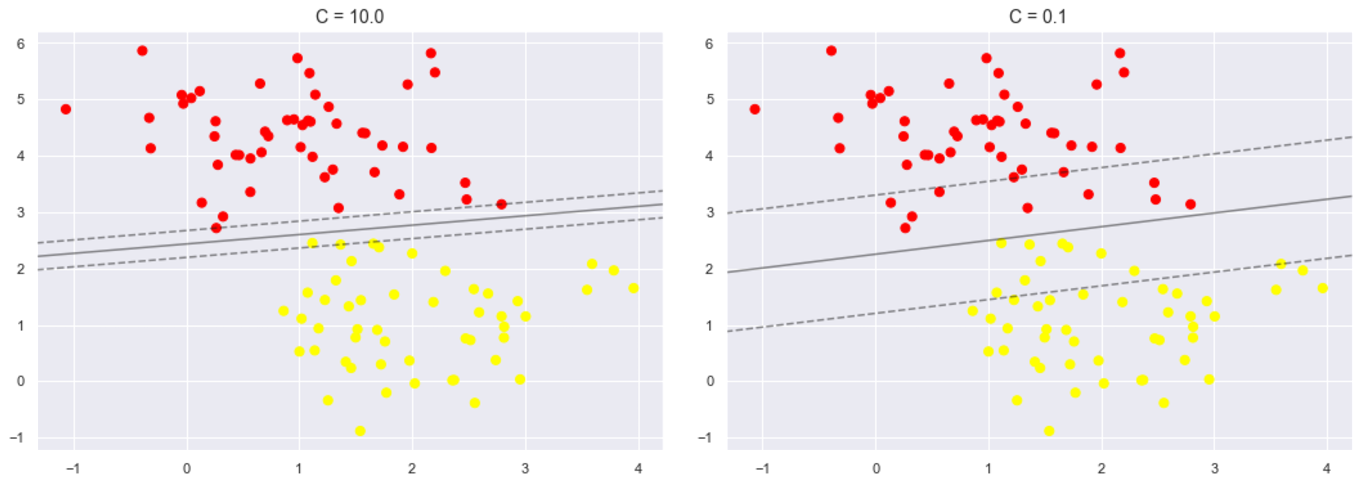
四、软间隔问题
软间隔问题主要是调节C参数, 当C趋近于无穷大时:意味着分类严格不能有错误, 当C趋近于很小的时:意味着可以有更大的错误容忍
X, y = make_blobs(n_samples=100, centers=2,
                  random_state=0, cluster_std=0.8)
plt.scatter(X[:, 0], X[:, 1], c=y, s=50, cmap='autumn');
先看看有噪声点的数据的分布
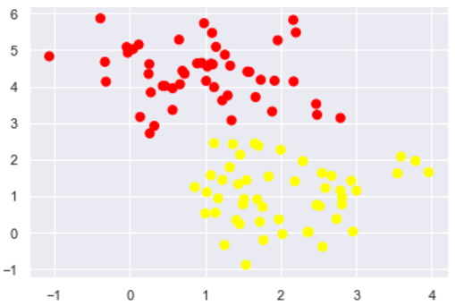
上面的分布看起来要严格地进行划分的话,似乎不太可能,我们可以进行软间隔调整看看
X, y = make_blobs(n_samples=100, centers=2,
                  random_state=0, cluster_std=0.8)

fig, ax = plt.subplots(1, 2, figsize=(16, 6))
fig.subplots_adjust(left=0.0625, right=0.95, wspace=0.1)

for axi, C in zip(ax, [10.0, 0.1]):
    model = SVC(kernel='linear', C=C).fit(X, y)
    axi.scatter(X[:, 0], X[:, 1], c=y, s=50, cmap='autumn')
    plot_svc_decision_function(model, axi)
    axi.scatter(model.support_vectors_[:, 0],
                model.support_vectors_[:, 1],
                s=300, lw=1, facecolors='none');
    axi.set_title('C = {0:.1f}'.format(C), size=14)
可以比较不同C参数模型地结果,在实际应用中可以适当调整以提高模型的泛化能力。
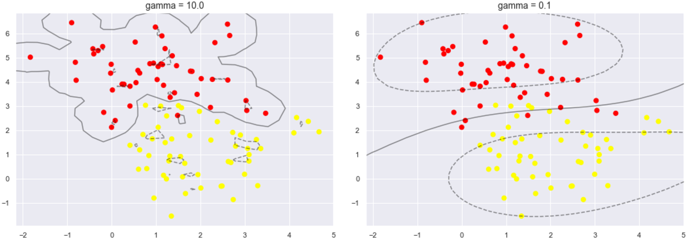
下面再看另一个参数gamma值,这个参数只是在高斯核函数里面才有。这个参数控制着模型的复杂程度,这个值越大,模型越复杂,值越小,模型就越精简。
X, y = make_blobs(n_samples=100, centers=2,
                  random_state=0, cluster_std=1.1)

fig, ax = plt.subplots(1, 2, figsize=(16, 6))
fig.subplots_adjust(left=0.0625, right=0.95, wspace=0.1)

for axi, gamma in zip(ax, [10.0, 0.1]):
    model = SVC(kernel='rbf', gamma=gamma).fit(X, y)
    axi.scatter(X[:, 0], X[:, 1], c=y, s=50, cmap='autumn')
    plot_svc_decision_function(model, axi)
    axi.scatter(model.support_vectors_[:, 0],
                model.support_vectors_[:, 1],
                s=300, lw=1, facecolors='none');
    axi.set_title('gamma = {0:.1f}'.format(gamma), size=14)
可以比较一下,当这个参数较大时,可以看出模型分类效果很好,但泛化不太好。当这个参数较小时,可以看出模型里面有些分类是有错误的,但是这个泛化能力更好,一般也应有的更多。
四、总结
通过这次简单的练习,对支持向量机模型有了更加深刻的理解,学习了在支持向量机中SVM的基本使用,以及软间隔参数的调整,还有核函数变化和gamma值等一些参数的比较。