python do Fourier transform

Fourier transform (FFT)

　　French scientist Fourier suggested that any one cycle curve, no matter how irregular or jumping, can be expressed as the superposition of a set of sine curves and smooth. I.e., the Fourier transform is an irregular curve broken down into a set of smooth sine curve process.

　　Object is the Fourier transform to convert the time domain signal (i.e., a time domain) to the frequency domain (i.e., frequency domain) on the signal , with the transform domain, for the same understanding of the angle of the thing will change, Therefore, in place of some bad time domain processing, processing can be relatively simple in the frequency domain . This signal processing can significantly reduce the amount of storage.

For example: playing the piano

Suppose there is a time domain function: y = f (x), in accordance with Fourier theory it can be decomposed into a series of superimposed sine function, their amplitudes A, frequencies ω initial phase or different φ:

$$ y = A_1sin (\ omega_1x + \ phi_1) + A_2sin (\ omega_2x + \ phi_2) + A_2sin (\ omega_2x + \ phi_2) + R $$

Therefore, the Fourier transform may convert a relatively complex function of a simple superposition of a plurality of functions, also the angle of approach to the frequency domain from the time domain, some of them deal with the problem it will be relatively simple.

Fourier transform of the correlation function

freqs = np.fft.fft.fftfreq (number of samples, the sampling period)　　is obtained by Fourier transform of the resulting sample number exploded sampling period frequency series array

np.fft.fft .fft (original sequence)　　the sequence of the original function of the value after the fast Fourier transform to obtain a complex arraymode is represented by the complex amplitude of the early phase of the complex argument representatives

np.fft.fft .ifft (complex sequence)　　complex array obtained through the inverse Fourier transform of the synthesized array of function values

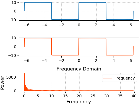
Case: the composite wave made for fast Fourier transform, to obtain an array of frequency decomposition wave amplitude, initial phase array, and draws an image in the frequency domain.

import numpy as np
import matplotlib.pyplot as plt
import numpy.fft as fft

x = np.linspace(-2 * np.pi, 2 * np.pi, 1000)

n = 1000
y = np.zeros(x.size)
for i in range(1, n + 1):
    y += 4 * np.pi / (2 * i - 1) * np.sin((2 * i - 1) * x)

complex_array = fft.fft(y)
print(complex_array.shape)  # (1000,) 
print(complex_array.dtype)  # complex128 
print(complex_array[0])  #(-2.1458390619955026e-12 is + 0j) 
y_new = fft.ifft (complex_array) 

plt.subplot ( 311 ) 
plt.grid (lineStyle = ' : ' ) 
plt.plot (X, Y, label = ' Y ' )   # Y is 1000 sinusoidal sequence summing 
plt.subplot (312 ) 
plt.plot (X, y_new, label = ' y_new ' , Color = ' OrangeRed ' )   # Y is ifft converted sequence 

# achieve frequency alignment decomposition wave 
freqs fft.fftfreq = (x.size, X [. 1] - X [0])
 # complex mode amplitude (magnitude of energy) signal 
complex_array = fft.fft(y)
pows = np.abs(complex_array)

plt.subplot(313)
plt.title('Frequency Domain', fontsize=16)
plt.xlabel('Frequency', fontsize=12)
plt.ylabel('Power', fontsize=12)
plt.tick_params(labelsize=10)
plt.grid(linestyle=':')
plt.plot(freqs[freqs > 0], pows[freqs > 0], c='orangered', label='Frequency') 
Plt.legend () 
plt.tight_layout () 
plt.show ()

Fourier transform based frequency domain filter

Noisy low-energy signal is an energy signal and the noise superimposed signal, a frequency domain filtering may be achieved by a Fourier transform noise.

By the FFT noise-containing signal into a frequency spectrum containing noise, low energy noise is removed, leaving a high-energy spectrum after leaving the high-energy signal through IFFT.

Case: removing noise (frequency domain filtering as an audio file based on Fourier transform noiseed.wav data set address ).

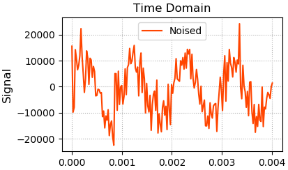
　　1, reads the audio file, an audio file obtaining basic information: the number of sampling, the sampling period, the value of each sampled audio signal. Rendering the audio time domain: time / displacement image

Import numpy AS NP
 Import numpy.fft AS NF
 Import scipy.io.wavfile AS WF
 Import matplotlib.pyplot AS PLT 

# reading audio file 
sample_rate, noised_sigs = wf.read ( ' ./da_data/noised.wav ' )
 Print (sample_rate )   # sample_rate: sampling rate 44100 
Print (noised_sigs.shape)     # noised_sigs: storing the audio samples for each sampling point displacement (220500,) 
Times = np.arange (noised_sigs.size) / sample_rate 

plt.figure ( ' the Filter ' ) 
plt.subplot ( 221 ) 
plt.title ( ' Time the Domain', fontsize=16)
plt.ylabel('Signal', fontsize=12)
plt.tick_params(labelsize=10)
plt.grid(linestyle=':')
plt.plot(times[:178], noised_sigs[:178], c='orangered', label='Noised')
plt.legend()

 

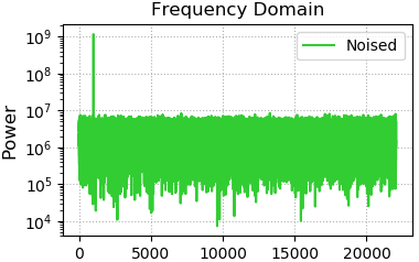
　　2, based on Fourier transform, obtaining the audio frequency domain information, rendering the audio frequency domain: frequency / energy image

# Fourier transformed, frequency domain images drawn 
freqs = nf.fftfreq (times.size, Times [. 1] - Times [0]) 
complex_array = nf.fft (noised_sigs) 
POWs = np.abs (complex_array) 

plt.subplot ( 222 ) 
plt.title ( ' Frequency the Domain ' , fontSize = 16 ) 
plt.ylabel ( ' the Power ' , 12 is fontSize = ) 
plt.tick_params (labelsize = 10 ) 
plt.grid (lineStyle = ' : ' )
 # exponential growth coordinates Paint 
plt.semilogy (freqs [freqs> 0], POWs [freqs> 0], C = ' LimeGreen', label='Noised')
plt.legend()

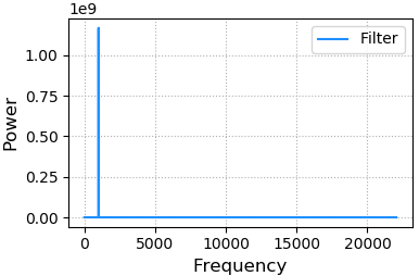
　　3, the low-frequency noise removing the audio frequency domain drawing: frequency / energy image

# Seeking maximum frequency energy value 
fund_freq = freqs [pows.argmax ()]
 # the WHERE function to find those who need to erase the plural index 
noised_indices = np.where (freqs! = Fund_freq)
 # copy of a copy of a complex array, to avoid contamination raw data 
filter_complex_array = complex_array.copy () 
filter_complex_array [noised_indices] = 0 
filter_pows = np.abs (filter_complex_array) 

plt.subplot ( 224 ) 
plt.xlabel ( ' Frequency ' , 12 is fontSize = ) 
plt.ylabel ( ' the Power ' , fontSize 12 is = ) 
plt.tick_params (labelsize = 10 )
plt.grid(linestyle=':')
plt.plot(freqs[freqs >= 0], filter_pows[freqs >= 0], c='dodgerblue', label='Filter')
plt.legend()

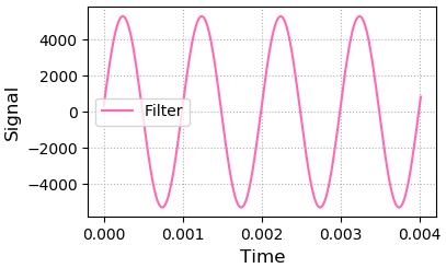
　　4, based on the inverse Fourier transform to generate a new audio signal, the audio rendering time domain: time / displacement image

filter_sigs = nf.ifft(filter_complex_array).real
plt.subplot(223)
plt.xlabel('Time', fontsize=12)
plt.ylabel('Signal', fontsize=12)
plt.tick_params(labelsize=10)
plt.grid(linestyle=':')
plt.plot(times[:178], filter_sigs[:178], c='hotpink', label='Filter')
plt.legend()

　　5, regenerate the audio file

# Audio file is generated 
wf.write ( ' ./da_data/filter.wav ' , sample_rate, filter_sigs) 
plt.show ()