Logistic regression -3. Decision boundary

Decision boundary

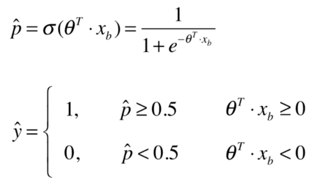
We can see different values of y determine boundary: \ [\ Theta ^ T \ cdot x_b = 0 \]
formula expression is a straight line, as the decision boundary, if a new sample, and after training to get the $ \ Theta $ multiplied, depending on whether greater than 0, determines which category in the end

Draw the decision boundary

If the sample has two characteristics \ (X1, X2 \) , then the decision boundary has: \ (\ theta_0 + \ theta_1 \ CDOT X1 + \ theta_2 \ CDOT X2 = 0 \) , determined \ (x2 = \ frac {- \ theta_0 - \ theta_1 \ cdot x1 } {\ theta_2} \)

# 定义x2和x1的关系表达式
def x2(x1):
    return (-logic_reg.interception_ - logic_reg.coef_[0] * x1)/logic_reg.coef_[1]
    
x1_plot = numpy.linspace(4,8,1000)
x2_plot = x2(x1_plot)

pyplot.scatter(X[y==0,0],X[y==0,1],color='red')
pyplot.scatter(X[y==1,0],X[y==1,1],color='blue')
pyplot.plot(x1_plot,x2_plot)
pyplot.show()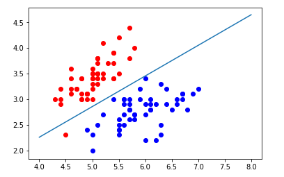

Decision to draw irregular borders

Feature field (for visualization, taking the characteristic value 2, i.e., rectangular region) in all the dot area visualization, see irregular decision boundary
function is defined for all points plotted domain features:

def plot_decision_boundary(model,axis):
    x0,x1 = numpy.meshgrid(
        numpy.linspace(axis[0],axis[1],int((axis[1]-axis[0])*100)),
        numpy.linspace(axis[2],axis[3],int((axis[3]-axis[2])*100))
    )
    x_new = numpy.c_[x0.ravel(),x1.ravel()]
    y_predict = model.predict(x_new)
    zz = y_predict.reshape(x0.shape)
    
    from matplotlib.colors import ListedColormap
    custom_cmap = ListedColormap(['#EF9A9A','#FFF59D','#90CAF9'])
    pyplot.contourf(x0,x1,zz,cmap=custom_cmap)

Drawing decision boundary logistic regression:

plot_decision_boundary(logic_reg,axis=[4,7.5,1.5,4.5])
pyplot.scatter(X[y==0,0],X[y==0,1],color='blue')
pyplot.scatter(X[y==1,0],X[y==1,1],color='red')
pyplot.show()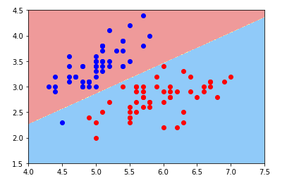

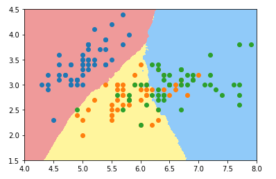
K-nearest neighbor algorithm to draw the boundaries of the decision:

from mylib import KNN

knn_clf_all = KNN.KNNClassifier(k=3)
knn_clf_all.fit(iris.data[:,:2],iris.target)

plot_decision_boundary(knn_clf_all,axis=[4,8,1.5,4.5])
pyplot.scatter(iris.data[iris.target==0,0],iris.data[iris.target==0,1])
pyplot.scatter(iris.data[iris.target==1,0],iris.data[iris.target==1,1])
pyplot.scatter(iris.data[iris.target==2,0],iris.data[iris.target==2,1])
pyplot.show()

k-nearest neighbor multi-classification (category 3) decision boundary in
taking k 3:00:

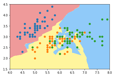
k takes 50:

Reference: Mu class notes