Questions asked

Two classes based on student achievement data and whether enrollment, students can successfully predict enrollment: use ex2data1.txtand ex2data2.txtdata, logistic regression and forecasting.

Data on the final edge.

ex2data1.txt processing

Scatter as seen, generally follow linear decision, but there are curved (non-linear), linear effect is not good, so two options are available: a program, no characteristic polynomial; Scheme II, there is a polynomial characteristics.

Scheme a: No characteristic polynomial

Ex2data1.txt data in logistic regression, no characteristic polynomial

Code is implemented as follows:

"""
    对ex2data1.txt中的数据进行逻辑回归（无多项式特征）
"""
from sklearn.model_selection import train_test_split
from matplotlib.colors import ListedColormap
from sklearn.linear_model import LogisticRegression
import numpy as np
import matplotlib.pyplot as plt
plt.rcParams['font.sans-serif'] = ['SimHei']  # 用来正常显示中文标签
plt.rcParams['axes.unicode_minus'] = False  # 用来正常显示负号

# 数据格式：成绩1,成绩2,是否被录取（1代表被录取，0代表未被录取）


# 函数（画决策边界）定义
def plot_decision_boundary(model, axis):
    x0, x1 = np.meshgrid(
        np.linspace(axis[0], axis[1], int((axis[1] - axis[0]) * 100)).reshape(-1, 1),
        np.linspace(axis[2], axis[3], int((axis[3] - axis[2]) * 100)).reshape(-1, 1),
    )
    X_new = np.c_[x0.ravel(), x1.ravel()]

    y_predict = model.predict(X_new)
    zz = y_predict.reshape(x0.shape)

    custom_cmap = ListedColormap(['#EF9A9A', '#FFF59D', '#90CAF9'])

    plt.contourf(x0, x1, zz, cmap=custom_cmap)

# 读取数据
data = np.loadtxt('ex2data1.txt', delimiter=',')
data_X = data[:, 0:2]
data_y = data[:, 2]

# 数据分割
X_train, X_test, y_train, y_test = train_test_split(data_X, data_y, random_state=666)

# 训练模型
log_reg = LogisticRegression()
log_reg.fit(X_train, y_train)

# 结果可视化
plot_decision_boundary(log_reg, axis=[0, 100, 0, 100])
plt.scatter(data_X[data_y == 0, 0], data_X[data_y == 0, 1], color='red')
plt.scatter(data_X[data_y == 1, 0], data_X[data_y == 1, 1], color='blue')
plt.xlabel('成绩1')
plt.ylabel('成绩2')
plt.title('两门课程成绩与是否录取的关系')
plt.show()

# 模型测试
print(log_reg.score(X_train, y_train))
print(log_reg.score(X_test, y_test))

Output:

0.8533333333333334
0.76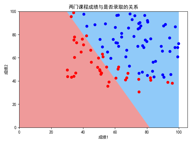

ex2data1 logistic regression (non-polynomial) .png

Option II: wherein introducing polynomials

Ex2data1.txt data in logistic regression, polynomial features introduced. After debugging, when 3, takes a long time for the degree; when the degree is 2, the acceptable time consuming, compared to the effect of a program with a lot better

To achieve the following:

"""
    对ex2data1.txt中的数据进行逻辑回归（引入多项式特征）
"""
from sklearn.model_selection import train_test_split
from matplotlib.colors import ListedColormap
from sklearn.linear_model import LogisticRegression
import numpy as np
import matplotlib.pyplot as plt
from sklearn.preprocessing import PolynomialFeatures
from sklearn.pipeline import Pipeline
from sklearn.preprocessing import StandardScaler
plt.rcParams['font.sans-serif'] = ['SimHei']  # 用来正常显示中文标签
plt.rcParams['axes.unicode_minus'] = False  # 用来正常显示负号

# 数据格式：成绩1,成绩2,是否被录取（1代表被录取，0代表未被录取）


# 函数定义
def plot_decision_boundary(model, axis):
    x0, x1 = np.meshgrid(
        np.linspace(axis[0], axis[1], int((axis[1] - axis[0]) * 100)).reshape(-1, 1),
        np.linspace(axis[2], axis[3], int((axis[3] - axis[2]) * 100)).reshape(-1, 1),
    )
    X_new = np.c_[x0.ravel(), x1.ravel()]

    y_predict = model.predict(X_new)
    zz = y_predict.reshape(x0.shape)

    custom_cmap = ListedColormap(['#EF9A9A', '#FFF59D', '#90CAF9'])

    plt.contourf(x0, x1, zz, cmap=custom_cmap)


def PolynomialLogisticRegression(degree):
    return Pipeline([
        ('poly', PolynomialFeatures(degree=degree)),
        ('std_scaler', StandardScaler()),
        ('log_reg', LogisticRegression())
    ])


# 读取数据
data = np.loadtxt('ex2data1.txt', delimiter=',')
data_X = data[:, 0:2]
data_y = data[:, 2]

# 数据分割
X_train, X_test, y_train, y_test = train_test_split(data_X, data_y, random_state=666)

# 训练模型
poly_log_reg = PolynomialLogisticRegression(degree=2)
poly_log_reg.fit(X_train, y_train)

# 结果可视化
plot_decision_boundary(poly_log_reg, axis=[0, 100, 0, 100])
plt.scatter(data_X[data_y == 0, 0], data_X[data_y == 0, 1], color='red')
plt.scatter(data_X[data_y == 1, 0], data_X[data_y == 1, 1], color='blue')
plt.xlabel('成绩1')
plt.ylabel('成绩2')
plt.title('两门课程成绩与是否录取的关系')
plt.show()

# 模型测试
print(poly_log_reg.score(X_train, y_train))
print(poly_log_reg.score(X_test, y_test))

Output is as follows :

0.92
0.92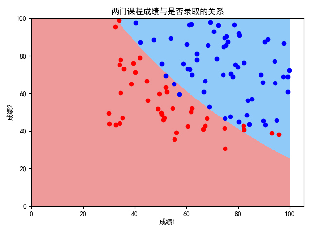

ex2data1 logistic regression (there is a polynomial) .png

ex2data2.txt processing

As a scatter plot shows that the decision boundary of this set of data is absolutely non-linear, polynomial introduced directly into the characteristics of the data ex2data2.txt in logistic regression.

Code is implemented as follows:

"""
    对ex2data2.txt中的数据进行逻辑回归（引入多项式特征）
"""
from sklearn.model_selection import train_test_split
from matplotlib.colors import ListedColormap
from sklearn.linear_model import LogisticRegression
import numpy as np
import matplotlib.pyplot as plt
from sklearn.preprocessing import PolynomialFeatures
from sklearn.pipeline import Pipeline
from sklearn.preprocessing import StandardScaler
plt.rcParams['font.sans-serif'] = ['SimHei']  # 用来正常显示中文标签
plt.rcParams['axes.unicode_minus'] = False  # 用来正常显示负号

# 数据格式：成绩1,成绩2,是否被录取（1代表被录取，0代表未被录取）


# 函数定义
def plot_decision_boundary(model, axis):
    x0, x1 = np.meshgrid(
        np.linspace(axis[0], axis[1], int((axis[1] - axis[0]) * 100)).reshape(-1, 1),
        np.linspace(axis[2], axis[3], int((axis[3] - axis[2]) * 100)).reshape(-1, 1),
    )
    X_new = np.c_[x0.ravel(), x1.ravel()]

    y_predict = model.predict(X_new)
    zz = y_predict.reshape(x0.shape)

    custom_cmap = ListedColormap(['#EF9A9A', '#FFF59D', '#90CAF9'])

    plt.contourf(x0, x1, zz, cmap=custom_cmap)


def PolynomialLogisticRegression(degree):
    return Pipeline([
        ('poly', PolynomialFeatures(degree=degree)),
        ('std_scaler', StandardScaler()),
        ('log_reg', LogisticRegression())
    ])


# 读取数据
data = np.loadtxt('ex2data2.txt', delimiter=',')
data_X = data[:, 0:2]
data_y = data[:, 2]

# 数据分割
X_train, X_test, y_train, y_test = train_test_split(data_X, data_y, random_state=666)

# 训练模型
poly_log_reg = PolynomialLogisticRegression(degree=2)
poly_log_reg.fit(X_train, y_train)

# 结果可视化
plot_decision_boundary(poly_log_reg, axis=[-1, 1, -1, 1])
plt.scatter(data_X[data_y == 0, 0], data_X[data_y == 0, 1], color='red')
plt.scatter(data_X[data_y == 1, 0], data_X[data_y == 1, 1], color='blue')
plt.xlabel('成绩1')
plt.ylabel('成绩2')
plt.title('两门课程成绩与是否录取的关系')
plt.show()

# 模型测试
print(poly_log_reg.score(X_train, y_train))
print(poly_log_reg.score(X_test, y_test))

Output:

The figure shows, better classification results.

0.7954545454545454
0.9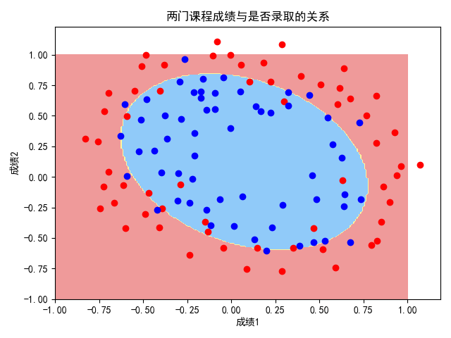

ex2data2 logistic regression (there is a polynomial) .png

Two data

ex2data1.txt

34.62365962451697,78.0246928153624,0
30.28671076822607,43.89499752400101,0
35.84740876993872,72.90219802708364,0
60.18259938620976,86.30855209546826,1
79.0327360507101,75.3443764369103,1
45.08327747668339,56.3163717815305,0
61.10666453684766,96.51142588489624,1
75.02474556738889,46.55401354116538,1
76.09878670226257,87.42056971926803,1
84.43281996120035,43.53339331072109,1
95.86155507093572,38.22527805795094,0
75.01365838958247,30.60326323428011,0
82.30705337399482,76.48196330235604,1
69.36458875970939,97.71869196188608,1
39.53833914367223,76.03681085115882,0
53.9710521485623,89.20735013750205,1
69.07014406283025,52.74046973016765,1
67.94685547711617,46.67857410673128,0
70.66150955499435,92.92713789364831,1
76.97878372747498,47.57596364975532,1
67.37202754570876,42.83843832029179,0
89.67677575072079,65.79936592745237,1
50.534788289883,48.85581152764205,0
34.21206097786789,44.20952859866288,0
77.9240914545704,68.9723599933059,1
62.27101367004632,69.95445795447587,1
80.1901807509566,44.82162893218353,1
93.114388797442,38.80067033713209,0
61.83020602312595,50.25610789244621,0
38.78580379679423,64.99568095539578,0
61.379289447425,72.80788731317097,1
85.40451939411645,57.05198397627122,1
52.10797973193984,63.12762376881715,0
52.04540476831827,69.43286012045222,1
40.23689373545111,71.16774802184875,0
54.63510555424817,52.21388588061123,0
33.91550010906887,98.86943574220611,0
64.17698887494485,80.90806058670817,1
74.78925295941542,41.57341522824434,0
34.1836400264419,75.2377203360134,0
83.90239366249155,56.30804621605327,1
51.54772026906181,46.85629026349976,0
94.44336776917852,65.56892160559052,1
82.36875375713919,40.61825515970618,0
51.04775177128865,45.82270145776001,0
62.22267576120188,52.06099194836679,0
77.19303492601364,70.45820000180959,1
97.77159928000232,86.7278223300282,1
62.07306379667647,96.76882412413983,1
91.56497449807442,88.69629254546599,1
79.94481794066932,74.16311935043758,1
99.2725269292572,60.99903099844988,1
90.54671411399852,43.39060180650027,1
34.52451385320009,60.39634245837173,0
50.2864961189907,49.80453881323059,0
49.58667721632031,59.80895099453265,0
97.64563396007767,68.86157272420604,1
32.57720016809309,95.59854761387875,0
74.24869136721598,69.82457122657193,1
71.79646205863379,78.45356224515052,1
75.3956114656803,85.75993667331619,1
35.28611281526193,47.02051394723416,0
56.25381749711624,39.26147251058019,0
30.05882244669796,49.59297386723685,0
44.66826172480893,66.45008614558913,0
66.56089447242954,41.09209807936973,0
40.45755098375164,97.53518548909936,1
49.07256321908844,51.88321182073966,0
80.27957401466998,92.11606081344084,1
66.74671856944039,60.99139402740988,1
32.72283304060323,43.30717306430063,0
64.0393204150601,78.03168802018232,1
72.34649422579923,96.22759296761404,1
60.45788573918959,73.09499809758037,1
58.84095621726802,75.85844831279042,1
99.82785779692128,72.36925193383885,1
47.26426910848174,88.47586499559782,1
50.45815980285988,75.80985952982456,1
60.45555629271532,42.50840943572217,0
82.22666157785568,42.71987853716458,0
88.9138964166533,69.80378889835472,1
94.83450672430196,45.69430680250754,1
67.31925746917527,66.58935317747915,1
57.23870631569862,59.51428198012956,1
80.36675600171273,90.96014789746954,1
68.46852178591112,85.59430710452014,1
42.0754545384731,78.84478600148043,0
75.47770200533905,90.42453899753964,1
78.63542434898018,96.64742716885644,1
52.34800398794107,60.76950525602592,0
94.09433112516793,77.15910509073893,1
90.44855097096364,87.50879176484702,1
55.48216114069585,35.57070347228866,0
74.49269241843041,84.84513684930135,1
89.84580670720979,45.35828361091658,1
83.48916274498238,48.38028579728175,1
42.2617008099817,87.10385094025457,1
99.31500880510394,68.77540947206617,1
55.34001756003703,64.9319380069486,1
74.77589300092767,89.52981289513276,1

ex2data2.txt

0.051267,0.69956,1
-0.092742,0.68494,1
-0.21371,0.69225,1
-0.375,0.50219,1
-0.51325,0.46564,1
-0.52477,0.2098,1
-0.39804,0.034357,1
-0.30588,-0.19225,1
0.016705,-0.40424,1
0.13191,-0.51389,1
0.38537,-0.56506,1
0.52938,-0.5212,1
0.63882,-0.24342,1
0.73675,-0.18494,1
0.54666,0.48757,1
0.322,0.5826,1
0.16647,0.53874,1
-0.046659,0.81652,1
-0.17339,0.69956,1
-0.47869,0.63377,1
-0.60541,0.59722,1
-0.62846,0.33406,1
-0.59389,0.005117,1
-0.42108,-0.27266,1
-0.11578,-0.39693,1
0.20104,-0.60161,1
0.46601,-0.53582,1
0.67339,-0.53582,1
-0.13882,0.54605,1
-0.29435,0.77997,1
-0.26555,0.96272,1
-0.16187,0.8019,1
-0.17339,0.64839,1
-0.28283,0.47295,1
-0.36348,0.31213,1
-0.30012,0.027047,1
-0.23675,-0.21418,1
-0.06394,-0.18494,1
0.062788,-0.16301,1
0.22984,-0.41155,1
0.2932,-0.2288,1
0.48329,-0.18494,1
0.64459,-0.14108,1
0.46025,0.012427,1
0.6273,0.15863,1
0.57546,0.26827,1
0.72523,0.44371,1
0.22408,0.52412,1
0.44297,0.67032,1
0.322,0.69225,1
0.13767,0.57529,1
-0.0063364,0.39985,1
-0.092742,0.55336,1
-0.20795,0.35599,1
-0.20795,0.17325,1
-0.43836,0.21711,1
-0.21947,-0.016813,1
-0.13882,-0.27266,1
0.18376,0.93348,0
0.22408,0.77997,0
0.29896,0.61915,0
0.50634,0.75804,0
0.61578,0.7288,0
0.60426,0.59722,0
0.76555,0.50219,0
0.92684,0.3633,0
0.82316,0.27558,0
0.96141,0.085526,0
0.93836,0.012427,0
0.86348,-0.082602,0
0.89804,-0.20687,0
0.85196,-0.36769,0
0.82892,-0.5212,0
0.79435,-0.55775,0
0.59274,-0.7405,0
0.51786,-0.5943,0
0.46601,-0.41886,0
0.35081,-0.57968,0
0.28744,-0.76974,0
0.085829,-0.75512,0
0.14919,-0.57968,0
-0.13306,-0.4481,0
-0.40956,-0.41155,0
-0.39228,-0.25804,0
-0.74366,-0.25804,0
-0.69758,0.041667,0
-0.75518,0.2902,0
-0.69758,0.68494,0
-0.4038,0.70687,0
-0.38076,0.91886,0
-0.50749,0.90424,0
-0.54781,0.70687,0
0.10311,0.77997,0
0.057028,0.91886,0
-0.10426,0.99196,0
-0.081221,1.1089,0
0.28744,1.087,0
0.39689,0.82383,0
0.63882,0.88962,0
0.82316,0.66301,0
0.67339,0.64108,0
1.0709,0.10015,0
-0.046659,-0.57968,0
-0.23675,-0.63816,0
-0.15035,-0.36769,0
-0.49021,-0.3019,0
-0.46717,-0.13377,0
-0.28859,-0.060673,0
-0.61118,-0.067982,0
-0.66302,-0.21418,0
-0.59965,-0.41886,0
-0.72638,-0.082602,0
-0.83007,0.31213,0
-0.72062,0.53874,0
-0.59389,0.49488,0
-0.48445,0.99927,0
-0.0063364,0.99927,0
0.63265,-0.030612,0

Author: @ smelly salted fish

Please indicate the source: https://www.cnblogs.com/chouxianyu/

Welcome to discuss and share!

sklearn combat logistic regression