Analysis of actual data (b)

Address data set extraction code: us2a

Age: 年龄，指登船者的年龄
Fare: 价格，指船票价格
Embark: 登船的港口

Q1: According to the port classification, various types of data obtained using python age, ticket price statistics (mean, variance, standard deviation, coefficient of variation)

import pandas as pd
data = pd.read_excel("D:\data\data.xlsx")

data = data.set_index("ID")

portS = data[data["Embarked"]=="S"]
portC = data[data["Embarked"]=="C"]
portQ = data[data["Embarked"]=="Q"]

portS_age = portS["Age"]
portS_fare = portS["Fare"]
portC_age = portC["Age"]
portC_fare = portC["Fare"]
portQ_age = portQ["Age"]
portQ_fare = portQ["Fare"]

port_details = pd.DataFrame({"均值":[portS_age.mean(),portC_age.mean(),portQ_age.mean(),portS_fare.mean(),portC_fare.mean(),portQ_fare.mean()],
            "方差":[portS_age.var(),portC_age.var(),portQ_age.var(),portS_fare.var(),portC_fare.var(),portQ_fare.var()],
            "标准差":[portS_age.std(),portC_age.std(),portQ_age.std(),portS_fare.std(),portC_fare.std(),portQ_fare.std()],
            "变异系数":[portS_age.mean()/portS_age.std(),portC_age.mean()/portC_age.std(),portQ_age.mean()/portQ_age.std(),portS_fare.mean()/portS_fare.std(),portC_fare.mean()/portC_fare.std(),portQ_fare.mean()/portQ_fare.std()]},
            index=['S港口年龄', 'C港口年龄', 'Q港口年龄', 'S港口票价', 'C港口票价', 'Q港口票价'])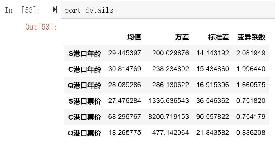

Q2: distribution image draw prices, which subject to verification data distribution (normal, chi-square, T)?

When random process known to be processed belongs to a family of a random process, the value may be employed to obtain the maximum likelihood estimation of the parameters

This part of the code reference in the Code by a group of big brother , really impressed with the code is very well written follow-up study to continue learning within the code details

Whether the normal distribution?

fare = data['Fare'].copy().values   # 单独选取fare列值
fare.sort()

loc, std = stats.norm.fit(fare)  # 最大似然求得均值与标准差
y = stats.norm.pdf(fare, loc=loc, scale=std)
plt.hist(fare, bins=10, density=True, label='Fare Distribution')
plt.plot(fare, y, color='#E78A61', label='normal fit')
plt.xlabel("Fare")
plt.ylabel("Density")
plt.title('Fare Distribution')
plt.legend()
plt.show()

norm_random = stats.norm.rvs(loc=loc, scale=std, size=len(fare))
norm_KS_stastic, norm_pvalue = stats.ks_2samp(fare, norm_random)
print("norm_KS_stastic = %.4f norm_pvalue = %.4f" % (norm_KS_stastic, norm_pvalue))
if(norm_pvalue<0.05):
    print("该分布不符合正态分布")
else:
    print("该分布符合正态分布")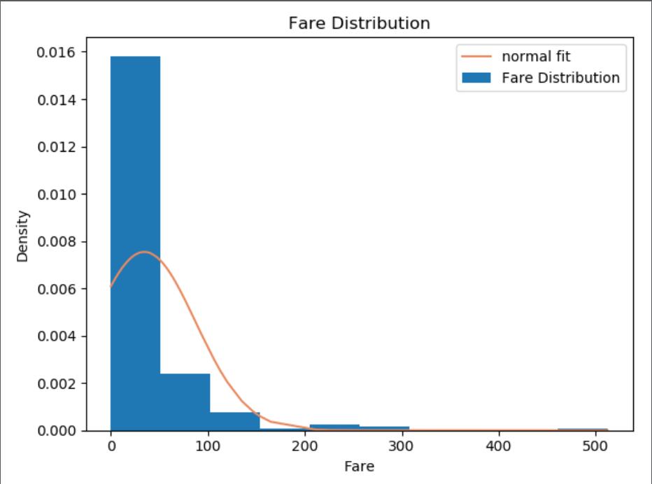

Whether or not in line with the chi-square distribution?

chi2_df,chi2_loc, chi2_std = stats.chi2.fit(fare)  # 最大似然求得均值与标准差
y = stats.chi2.pdf(fare, df=chi2_df, loc=chi2_loc, scale=chi2_std)
plt.hist(fare, bins=10, density=True,label='Fare Distribution')
plt.plot(fare, y, color='#E78A61', label='chi2 fit')
plt.xlabel("Fare")
plt.ylabel("Density")
plt.title('Fare Distribution')
plt.legend()
plt.show()

chi2_random = stats.chi2.rvs(df=chi2_df,loc=chi2_loc, scale=chi2_std, size=len(fare))
chi2_KS_stastic, chi2_pvalue = stats.ks_2samp(fare, chi2_random)
print("chi2_KS_stastic = %.4f chi2_pvalue = %.4f" % (chi2_KS_stastic, chi2_pvalue))
if(chi2_pvalue<0.05):
    print("该分布不符合卡方分布")
else:
    print("该分布符合正态分布")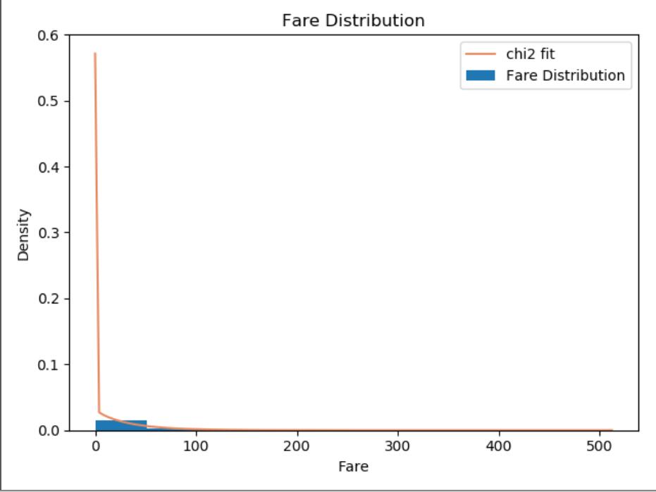

Whether the distribution of T?

t_df, t_loc, t_std = stats.t.fit(fare)  # 最大似然求得均值与标准差
y = stats.t.pdf(fare,df=t_df, loc=t_loc, scale=t_std)
plt.hist(fare,bins=10, density=True, label='Fare Distribution')
plt.plot(fare, y, color='#E78A61', label='t fit')
plt.xlabel("Fare")
plt.ylabel("Density")
plt.title('Fare Distribution')
plt.legend()
plt.show()

norm_random = stats.t.rvs(df=t_df,loc=t_loc, scale=t_std, size=len(fare))
t_KS_stastic, t_pvalue = stats.ks_2samp(fare, norm_random)
print("t_KS_stastic = %.4f t_pvalue = %.4f" % (t_KS_stastic, t_pvalue))
if(t_pvalue<0.05):
    print("该分布不符合T分布")
else:
    print("该分布符合正态分布")

Final analysis

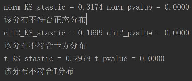
The distribution does not meet any of these three

Q3: the price difference between the ports of S and Q meets certain distribution?

s_fare = portS_fare.copy().values
q_fare = portQ_fare.copy().values

mean2 = s_fare.mean()-q_fare.mean()
std2 = (s_fare.std()**2/len(s_fare)+q_fare.std()**2/len(s_fare))**0.5

x = np.arange(- 40, 40)
y = stats.norm.pdf(x, mean2, std2)

plt.plot(x, y)
plt.xlabel("S_Fare - Q_Fare")
plt.ylabel("Density")
plt.show()

The image shows the difference between the two ports subject to the normal cost of approximately