Title name of the chaos to take, Tucao about "preliminary elementary number theory," the name.
The concept of a network flow
1.1 introduced
"Distribution" is the production life of a class of common problems. How to allocate only the best, there is a problem technical content.
For the "optimal allocation" problem, dynamic programming is an effective solution. However, some can not assign an accurate description of the "decision-making", "state", "phase" profile. Here we look at such a simple question:
A research study team received a topic contains 25 tasks within the group, a total of A, B, C, D, E five students. They work attitude and work efficiency (up to how many are willing to do the task) are different, as follows:
Full name Maximum number of tasks Consuming a single task Armor 4 42min B 5 56min Propionate 6 71min Ding 7 108min Amyl 8 121min
Assuming that the task can not be done at the same time, the minimum time required to complete all required tasks.
This problem does not seem easy to use dynamic programming. Previous \ (i \) personal order division stage? It does not seem right. Relationships between people here do not seem to.
This problem can be multi-dimensional linear programming to do, you can also consider using network flow to resolve. This is an important graph theory algorithms.
For the convenience of description, select a leader. Let's look at this simple flow chart:
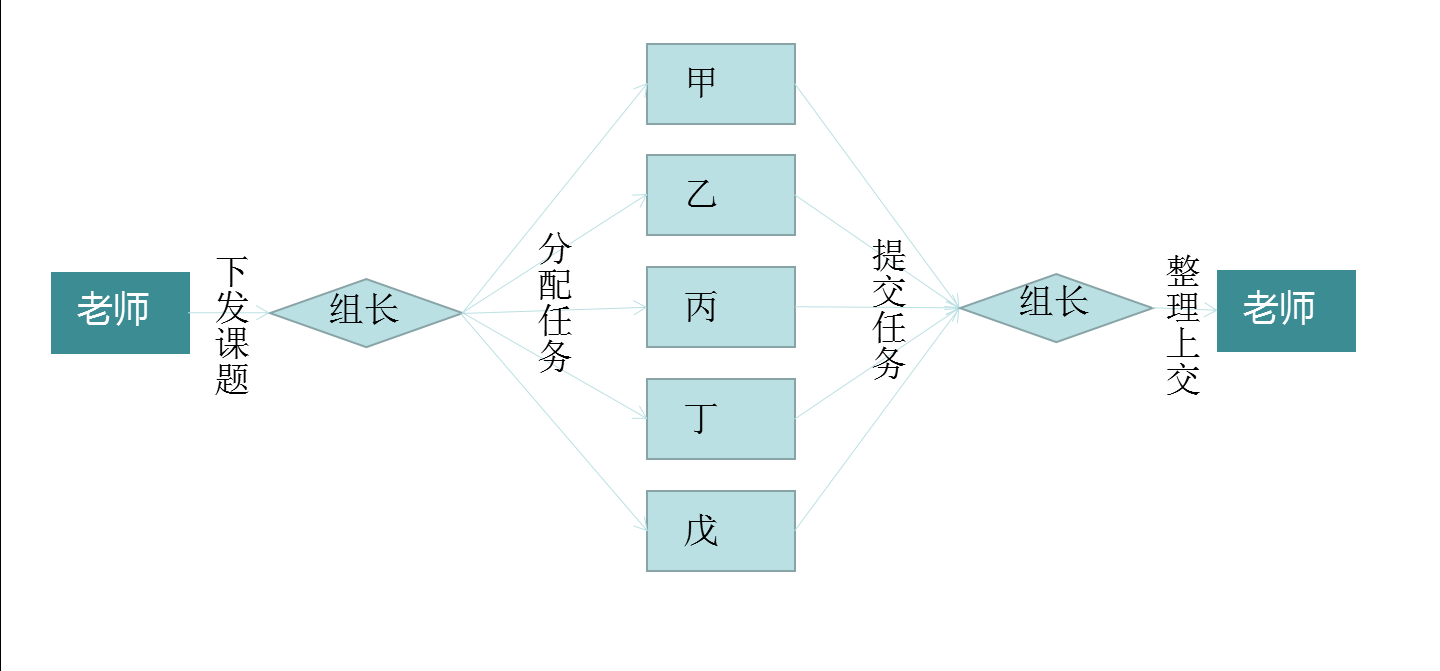
This is like a flow chart of a production line, 25 tasks from the teacher there, and finally back to the teacher to go there. Of course, to go back to that task.
Allocation may be made to the following task:
As shown, each of the arrows marked on the task assigned to each person, took a total of 33 hours 13 minutes.
You can see, if everyone as a node, then the only person responsible for "processing" tasks, not "store" mission. This is a very important feature. Furthermore, we can extract the mathematical model of them.
1.2 Definitions
一个网络\(G\)是一个有向图,其每一条边\((x,y)\)可以用一个非负数\(c(x,y)\)表示这条边的“容量”(capacity)。规定如果\((x,y)\)不是这个图中的边,则\(c(x,y)=0\)。有些时候,网络中的边又叫做弧。
每一个这样的网络中都有两个特殊的节点:源点\(S\)和汇点\(T\)。
设函数\(f(u,v)\)是作用在边\((u,v)\)上的函数,满足:
1.\(f(u,v) \leq c(u,v)\)
2.\(f(u,v) = -f(v,u)\)
3.\(\forall x\neq S, x \neq T, \sum f(u,x) = \sum f(x,v)\)
那么称\(f\)是网络\(G\)的一个流函数。对于一个边\((u,v)\),\(f(u,v)\)就是它的流量。
以上这三个性质分别称为容量限制,斜对称,流量守恒。请结合“水流”和“河道”的关系加强理解:水流不会超过河道,且不可压缩。
容量限制还有非常棒的一点:它省去了我写\(\sum\)下标的麻烦,因为不在边上的流量一定是\(0\)。(当然,这样做未必标准规范。)
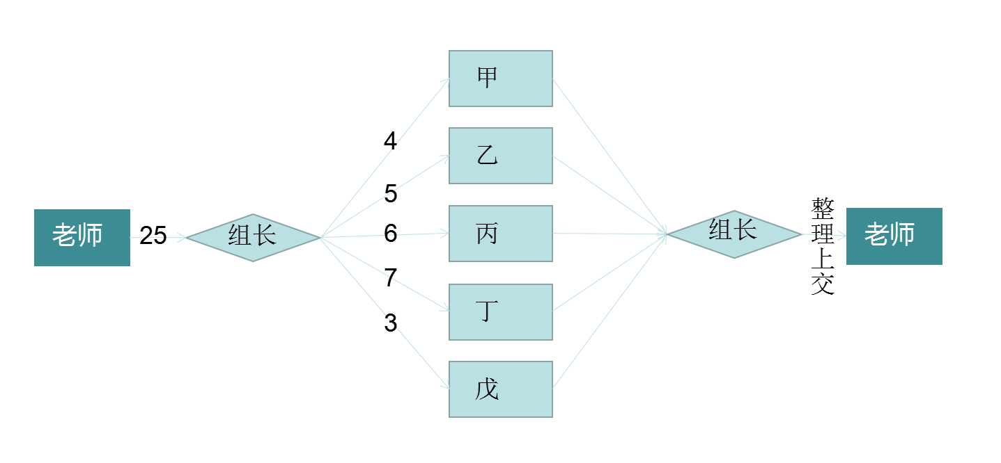
在上面的任务分配中,从“组长”到“甲”的流量为\(4\),从“组长”到“乙”的流量为\(5\),以此类推。
源点\(S\)和汇点\(T\)比较特殊,它们可以“发送”和“储存”流量。源点向整个网络运输的流量就是整个网络的流量,大小为\(\sum f(S,v)\)。
网络流还有一个有趣的性质:选取一个不含源点、汇点的点集,这个点集也满足流量平衡!这个性质可以看做是高斯定理的“离散版本”,在之后的网络流建模中会有所体现。
网络流的思想非常巧妙;正因如此,用网络流解题不像其他数据结构,是需要花费一点心思的。如何构建网络?如何转换问题?这些都是需要考虑的。
2 有关算法
2.1 最大流算法
网络中的最大流量就叫最大流。一个网络的流函数有很多;但幸运的是,我们可以避免直接对流函数操作,采用一种巧妙的方法。
2.1.1 Edmonds-Karp增广路算法
我们关注源点发送的其中一股流量。这股流量通过一条路径,最终流向了汇点。这样的路径叫做增广路。不难想到,路上的流量\(f\)等于路上容量的最小值\(\min c\)。
仔细一想,是不是源点发送的流量都会经过若干条增广路,然后全部流向汇点?我们只要尽可能地找出增广路,就可以求出最大流了!
这就是Edmonds-Karp算法的雏形了。通过BFS,我们可以找到一条增广路,并求出这条路上的流量。如何再找出一条增广路呢?再做一次BFS会返回同样的路径,而直接维护边上的信息又不太方便。
我们考虑直接修改增广路上的容量:求出流量\(f\)后,对路上的每一条边\((x,y)\),都执行\(c(x,y)=c(x,y)-f\),防止新的增广路超过容量。请注意,在原来流量\(f\)的基础上,我们还可能构造一个“逆流”\(f'\),使得某个\(f(x,y)\)直接与\(f'(x,y)\)抵消了。这样做是可行的,需要考虑。
通过执行\(c(x,y)-=f\),\(c(y,x)+=f\)后,得到的新网络叫做残量网络。在这个网络上添加的流量,一定不会超过原来的容量。
In summary, the BFS + form configured to detect the remaining amount of the network, we can obtain, respectively, a plurality of possible traffic \ (F, F ', F' ', \ cdots \) ; the maximum flow is obtained by adding the entire network .
The first is the search for augmenting paths part:
inline bool find_argumenting_path()
{
    memset(visit, 0, sizeof(visit));//标记
    queue<int> q; q.push(S); inq[S] = Inf; visit[S] = true;

    while(!q.empty())
    {
        int cur = q.front(); q.pop();
        for(rg int e = head[cur]; e; e = edge[e].next)
        {
            if(edge[e].capacity <= 0)
                continue;

            int to = edge[e].to;
            if(visit[to] == true)
                continue;

            inq[to] = min(inq[cur], edge[e].capacity);
            pre_edge[to] = e;//标记边,方便记录路径
            q.push(to); visit[to] = true;
            if(to == T)
                return true;
        }
    }
    return false;
}
We note that here we use an inqarray that represents the "residual flow of a node." It can be understood: we inject enough water at the source point, when water flows along the edge, which must receive side limit capacity. The final amount of water reaching the meeting point of this is that we need to increase traffic. Thus, for the edge \ ((X, Y) \) , there must be inq[y]=min(inq[x], edge[e].capacity).
Once you find an augmenting path, we will answer to this is added to the flow, and updates the residual network:
inline void update()
{
    int cur = T;
    while(cur != S)
    {
        int e = pre_edge[cur];
        edge[e].capacity -= inq[T];
        edge[e^1].capacity += inq[T];
        cur = edge[e].front;
    }
    max_flow += inq[T];
}
The previous premarker, we can restore a path from S to T, and the capacity adjustment on the side of the path.
Finally, the code in the main program as follows:
while(find_argumenting_path() == true)
    update();