Descriptive statistics data
A note, at least I'm still trying
table of Contents:
Central tendency of the data:
- The mode, median, mean, quantile, poor
- Arithmetic mean, weighted mean, geometric mean
Data from the trend:
- Numerical data: variance, standard deviation, range, mean difference
- Sequence data: interquartile
- Category Data: iso ratio of all the
The relative degree of dispersion:
- Coefficient of variation
Shape of the distribution:
- Skewness, kurtosis coefficients
Descriptive statistics charts or by means of numerical summary of statistical tools to describe data
(All code is based on python)
1. The central tendency of the data:
The mode : frequency is highest values occur in a set of data
1 mode(data)
Median : sort the data in the data after the centered position
median(data)
Average : All data is divided by the sum of the number of data
mean(data)
Quantile : i.e. sub-sites, refers to the probability distribution of a random variable data points into several aliquots, commonly used median (i.e., binary digits), quartiles, percentiles number, etc.
# The data packet by df1 and df2 PD
Grouped = data.groupby ([ ' df1 ' , ' df2 ' ])
 # by calculation of 40% quantile quantile
Grouped [ ' GMV ' ] .quantile (0.4)

#numpy
s1 = array(data['df3'])
np.percentile(s1,0.4)
Poor : also known as an error or a full-pitch range (the Range), represented by R, it is used to represent the variation in the number of statistics (measures of variation), which is the gap between the maximum and minimum values, i.e., the maximum value minus the resulting data of the minimum value
ptp(data)
Arithmetic Mean : Mean number of entries that the resulting data by dividing the algebraic sum of a data set
Geometric mean : the N is even N-th root of the product of open data, (x1 * x2 * x3 * ... * xn) ^ (1 / n). And the geometric mean of a set of numbers is not larger than the arithmetic mean constant! (X1 * x2 * x3 * ... * xn) ^ (1 / n) ≤ (x1 + x2 + x3 + ... + xn) / n
Weighted average of : the original data is calculated in accordance with a reasonable proportion ( weight is proportional share )
Such as: if the number n, x1 f1 occurs once, x2 appears times f2, ..., fk XK appears times, then (x1f1 + x2f2 + ... xkfk) / (f1 + f2 + ... + fk) is called x1 , x2, ..., xk weighted average. f1, f2, ..., fk are x1, x2, ..., xk the right.
2. Data from the trend:
Numerical data:
Variance : is a measure of probability theory and statistical variance or a set of random variables discrete level metrics. Variance is a measure of probability theory and its mathematical expectation of a random variable (ie mean) between the degree of deviation. The statistical variance (sample variance) is the difference between the respective data thereto respectively and the average of the average square. Research variance that is, the degree of deviation is of great significance.
 or
or 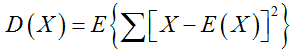
was (data)
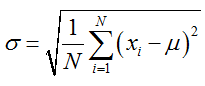
Standard deviation : Unit Standard value and its overall average of each of the squared deviations of the square root of the arithmetic mean. The variance of the data we are dealing with the dimension is inconsistent, although that best describes the degree of deviation from the mean of the data, but the processing results are not consistent with our intuitive thinking.
std(data)
Mean difference : one is represented by the degree of difference between the value of each variable value. It refers to the arithmetic mean value of each variable with the absolute value of the average deviation.
The average differences, the greater the degree of difference flags indicate the arithmetic mean value, the less representative of the arithmetic mean; mean difference is smaller, the smaller the degree of difference indicates that the arithmetic mean value of each marker, the Arithmetic the average representative will be. Due to the deviation becomes zero, the mean deviation and the deviation can not be divided by the number obtained from the difference, and to eliminate the sign must be taken away from the absolute difference. Mean difference of the average difference between the reaction and the arithmetic mean value of each flag.
Mean square error :
It reflects the mean squared error estimate is a measure of the degree of difference between the estimated amount, in other words, the difference between the square of the parameter value and the true value of the parameter estimates expected value. MSE data can be evaluated the degree of change, the smaller the MSE value is, the predictive model described the experimental data with better accuracy
Covariance:
Covariance is a measure of the overall error of two variables. Is a special case of the variance-covariance, i.e., when the two variables are the same situation. Covariance represents the overall error in two variables, which only represents a different variable error variance. If the trends of the two variables the same, that is to say if one is greater than their expectations, the other is also larger than its own expectations, then the covariance between the two variables is positive. If the two variables opposite trend, i.e., wherein a is greater than its desired value, but less than a further desired value itself, then the covariance between the two variables is negative.
Sequence data :
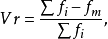
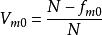
Interquartile range : is the upper quartile (Q3, which is located 75%) as a difference between the lower quartile (Q1, which is located 25%).
 Which
Which
 Which
Which ![]() represents the ratio of all the different,
represents the ratio of all the different, ![]() represents a mode number, N denotes the total number of overall unit (i.e., the number of overall)
represents a mode number, N denotes the total number of overall unit (i.e., the number of overall)
3, the relative degree of dispersion:
Dispersion coefficient : also known as the coefficient of variation. Dispersion coefficient is a measure of the relative degree of dispersion of statistic data, mainly for comparing different degree of dispersion of sample data. Dispersion coefficient, indicating the degree of dispersion of data is large; small dispersion coefficient, indicating the degree of dispersion of data is small.
Dispersion coefficient is a measure of the value of a statistic degree of dispersion of data in each observation. When comparing two or more discrete level information, and if the average number of units of measure the same, standard deviation can be directly compared. If the unit and (or) average number is not the same, comparing the degree of dispersion can not use standard deviation, and standard deviation for an average ratio (relative value) employed to compare. 
![]() It represents the overall sample dispersion coefficient and dispersion coefficient
It represents the overall sample dispersion coefficient and dispersion coefficient
In probability theory and statistics, the coefficient of variation (coefficient of variation), a discrete probability distribution is a normalized level measurement, defined as the standard deviation ![]() from the mean
from the mean ![]() than the
than the
 Dispersion coefficient (coefficient of variation) is defined only in the average value is not zero, but generally applies to the average value is greater than zero. Also known as the coefficient of variation from standard units or slip risk.
4, the distribution shape:
Skewness: also known as the coefficient of variation, indicating the degree of asymmetry of the statistical parameters assigned random sequence, represented by Cs. And Cv only reflect the average case and discrete frequency distribution curve of the degree of density, but does not reflect its symmetry (i.e., skewed) case, it is necessary to introduce a further parameter, i.e. the deviation coefficient Cso. The larger the absolute value of the skewness, the more highly skewed.
偏态系数以平均值与中位数之差对标准差之比率来衡量偏斜的程度,用SK表示偏斜系数:偏态系数小于0,因为平均数在众数之左,是一种左偏的分布,又称为负偏。偏态系数大于0,因为均值在众数之右,是一种右偏的分布,又称为正偏。
简单偏态系数: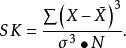
加权偏态系数: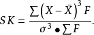
左右不对称即为偏态 。口诀一:看长尾在哪边就是往哪偏。口诀二:峰左移,右偏态;峰右移,左偏态
偏态系数绝对值值越大,偏斜程度越厉害。SK< 0 左偏SK> 0 右偏。SK以mean、mode之差与σ的比例来计算的,因此mean>mode,也就是右偏的时候,SK>0
峰态系数:
用来反映频数分布曲线顶端尖峭或扁平程度的指标。有时两组数据的算术平均数、标准差和偏态系数都相同,但他们分布曲线顶端的高耸程度却不同
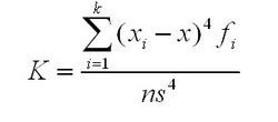 峰度系数可以为负数
正态分布的峰度K=3,均匀分布的峰度K=1.8。kurtosis=K-3 称为超值峰度。kurtosis>0,尖峰态(leptokurtic),数据集比较分散,极端数值较多。kurtosis<0,低峰态(platykurtic),数据集比较集中,两侧的数据比较少
个人笔记。。。