Spatial filtering base

Spatial correlation and convolution

dev_close_window ()
dev_open_window (0, 0, 512, 512, 'black', WindowHandle)

read_image(Image, 'convolution')

f:= [3, 3, 3, 0, 0, 0, 1, 1, 1, 0, 0, 0]
convol_image(Image, ImageResult, f, 'mirrored')

f1:= [3, 3, 3, 0, 1, 0, 0, 1, 0, 0, 1, 0]
convol_image(Image, ImageResult1, f1, 'mirrored')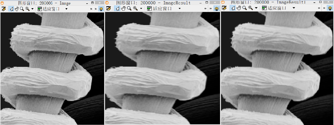

Left to right are the original image, and using the result of f f1 after convolution. Details of the two can be seen more clearly in FIG horizontal, vertical and blurred detail, FIG. 3 -phase.

Mean Filter

To achieve a smooth image.
An arbitrary position in the image (x, y) is the average value of the gradation (x, y) is the gradation value of 9 3 * 3 neighborhood divided by the center and 9.
According to this definition, the operator may be implemented using convol_image mean filter:

f3 := [3, 3, 9, 1, 1, 1, 1, 1, 1, 1, 1, 1]
convol_image(Image, ImageResult3, f3, 'mirrored')

In addition, a directly HALCON mean filter, the same effect can be achieved:

mean_image(Image, ImageMean, 3, 3)

Spatial smoothing filter

Removing an image for some trivial details, and bridging a gap in a line or curve goals before extraction.

Linear smoothing filter
mean filter is a low pass filter.
Noise reduction principle: typical random noise from the composition abrupt change in gray level, thus smoothing the noise can be reduced. However, due to the image edge it is also the case, mean filter can cause negative effects of blurring the edges.
Weighted mean filter coefficients of the filter 1 is incomplete, for example, such a filter:
\ [\ FRAC {1} {16} \ left [\} the begin {Matrix 1 & 2. 4 & 1 & 2 & 2 \\ \\ 1 & 2 & 1 \ end {
matrix} \ right] \] template size which is determined by the coming into the background of the size of the object
Sorting statistics (non-linear) filters
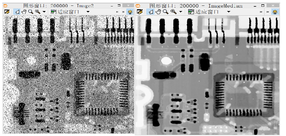
median filter processing impulse noise (salt and pepper noise), such noise is superimposed in the form of black and white dots on the image. The dots have different gray looks closer to its neighboring points.

median_image(Image2, ImageMedian, 'circle', 2, 'mirrored')

Median filtering a radius do circular filter 2:

Sharpening spatial filter

The first derivative:
\ [\ FRAC {\ partial F} {\ partial X} = F (X +. 1) - F (X) \]
second order differential
\ [\ frac {\ partial ^ {2} f} {\ partial x ^ {2}} =
f (x + 1) + f (x - 1) - 2f (x) \] digital image edge transitions of the gray ramp is similar, since the ramp is a non-zero order differential , the first derivative will produce thicker edges. Zero second order differential is produced by a separate double-pixel-wide edge;
Thus, a second differential good order differential than in enhancing detail, is a desirable feature for image sharpening.

Laplace operator

Isotropic filter independent mutations direction of the image in response to the filter effect of the filter is rotationally invariant, i.e., rotation of the original image after the filtering process gives the same result as a result of rotation of the first filter then obtained.
Laplacian
\ [\ nabla ^ {2} f = \ frac {\ partial ^ {2} f} {\ partial x ^ {2}} + \ frac {\ partial ^ {2} f} {\ partial y ^ {2}} \
] for the two-dimensional image F (x, y), respectively, seek second partial derivatives in the x, y directions, two discrete variables derived Laplacian is:
\ [ \ nabla ^ {2} f ( x, y) = f (x + 1, y) + f (x - 1, y) + f (x, y + 1) + f (x, y -1) - 2f (x, y) \]
template filter:

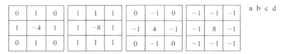
a filter template is to achieve the above operator used, b is made a diagonal extension, c and d are the a and b -1 is multiplied.
Laplacian image and the original image superposition, contextual characteristics can be restored and maintained Laplacian sharpening effect can be expressed as:
\ [G (X, Y) = F (X, Y) + C [\ nabla ^ {2} f
(x, y)] \] when using a template or b, c = -1, when using c or d, c = 1. Look central coefficient is positive or negative.
Halcon can be used directly in the corresponding template do convolution:

f := [3, 3, 1, 0, 1, 0, 1, -4, 1, 0, 1, 0]

convol_image(Image, ImageResult, f, 'mirrored')

* 将拉普拉斯变换后的图像与原图像叠加，得到锐化后的图像
abs_diff_image(Image, ImageResult, ImageAbsDiff, 1)

There halcon laplace defined template, to replace f 'laplace4',
in addition to direct defined Laplacian laplace.

Unsharp masking and filtering high lift

Unsharp masking is subtracted from the original image in the original image to obtain smoothed a template, and added to the original image.
Order \ (f \ overline (x, y) \) represents a blurred image, unsharp masking to equation:
Template:
\ [G_ mask} {(X, Y) = F (X, Y) - F \ overline ( x, y) \]
plus a weighted portion of the template in the original:
\ [G (X, Y) = F (X, Y) + K * G_ {mask} (x, y) \]
When the weighting coefficients when k = 1, the above definitions are called unsharp masking; k> 1, referred to as a high lift filter; k <1 does not emphasize the contribution of unsharp template.

dev_close_window ()

dev_open_window (0, 0, 512, 512, 'black', WindowHandle)
 
read_image(Image, 'dipxe_text')

* 高斯滤波器平滑
gauss_filter(Image, ImageGauss, 3)

* 和原图相减
sub_image(Image, ImageGauss, ImageSub, 1, 0)

* 线性变换，令k=4.5
scale_image(ImageSub, ImageScaled, 4.5, 0)

* 图像叠加
add_image(Image, ImageScaled, ImageResult, 1, 0)

Figure on hold, and drawing on the book are used to achieve a bit.

Using a nonlinear first-order differential image sharpening - Gradient

Sobel operator
Robert cross gradient operator

Feeling a little efficiency decreased. . . . Tomorrow to make a summary of this chapter after the reading, what kind of image type and what kind of filter processing, probably explain why.

Used Halcon operator

convol_image (Image, ImageResult, FilterMsk, Margin): specified convolution kernel FilterMask convoluting.
FilterMask may be already defined in a file, you can also write your own a matrix, written tuple: [MaskHeight, MaskWidth, Weight , V1, V2]
for example (common Gaussian filter): \
[\ {FRAC 1} {16} \ left [
\ begin {matrix} 1 & 2 & 1 \\ 2 & 4 & 2 \\ 1 & 2 & 1 \ end {matrix} \ right] \] written tuple: [3, 3, 16, 1, 2, 1, 2, 4, 2, 1, 2, 1]
written in a file (not tried):
. 3. 3
16
1 2 1
2 4 2
1 2 1
mean_image (Image, ImageMean, MaskWidth, MaskHeight): Use width MaskWidth, the height of the convolution kernel MaskHeight mean filter
median_image (Image, ImageMedian, MaskType, Radius, Margin): median filter, radius Radius shape using median filtering as a filter MaskType
laplace (Image, ImageLaplace, Result, MaskSize, FilterMask): Laplace operator
gauss_filter (Image, ImageGauss, Size): Specifies the Gaussian filter Size
roberts (Image, ImageRoberts, FilterType): Robert was found with the image edge filter
sobel_amp (Image, EdgeAmplitude, FilterType, Size): found using image edge Sobel filter, the filter matrix as the template using the following two:
\ [A = \ left [\} the begin {Matrix. 1 & 2. 1 & & \\ 0 0 & 0 \\ -1 & -2 & -1 \ end {matrix} \ right] \]

\[ B = \left[ \begin{matrix} 1 & 0 & -1 \\ 2 & 0 & -2 \\ 1 & 0 & -1 \end{matrix} \right] \]

Image processing notes (seven)