
DolphinDB is a high-performance distributed time-series database with distributed computing, transaction support, multi-mode storage, and streaming-batch integration capabilities. It is very suitable as an ideal lightweight big data platform to easily build a one-stop high-performance real-time database. database.
This tutorial will use cases and scripts to introduce how to quickly build a real-time data warehouse through DolphinDB to help various industries (such as energy and power, aerospace, Internet of Vehicles, petrochemicals, mining, intelligent manufacturing, trade and government affairs, finance, etc.) Quickly implement low-latency complex indicator calculation and analysis of massive data in business scenarios.
This tutorial includes an introduction to principles and practical operations, as well as supporting sample code. Users can follow the tutorial and combine their own business characteristics to build a lightweight and high-performance real-time data warehouse .
1 Introduction
1.1 Case background and needs
With the advent of the big data era, all walks of life have increasingly higher requirements for real-time and accuracy of data processing. Although traditional offline data warehouses can meet the data storage and offline analysis needs of enterprises to a certain extent, they are often unable to handle large-scale real-time data. Especially in leading Internet of Things and financial companies that have very high requirements for real-time data, the limitations of offline data warehouses are even more obvious.
Taking power plants in the electric power industry as an example, each power plant has a large number of measuring points that collect the operating data of the power plant in real time. How to combine massive power plant operation data and conduct accurate and complex calculations and analysis of real-time data has become a major challenge for power plants. Traditional real-time databases lack aggregate analysis and computing capabilities for massive data, while offline data warehouses built by traditional big data systems are difficult to meet deeper business needs due to slow processing speed, high latency, and complex architecture.
As a lightweight one-stop real-time data warehouse solution, DolphinDB has become the solution to this problem with its high-performance distributed computing framework, real-time streaming data processing capabilities, distributed multi-modal storage engine and memory computing technology. Ideal.
This article will use DolphinDB to implement a typical power generation side demand scenario. With 40,000 measuring points sampling every second on the power generation side, various measuring point indicators (maximum value, Minimum value, average value, median, 95% quantile, 5% quantile, change amount, change rate, start value, end value, etc.), and achieve millisecond-level query response. These indicators are crucial for power station operation monitoring, fault warning, energy efficiency analysis, big data display, etc. (For more IoT industry scenario solutions, please add DolphinDB assistant dolphindb1)
1.2 Basic concepts of data warehouse
Data Warehouse (DW or DWH for short) is a system used to store, process and analyze large amounts of data, designed to support the decision-making process in specific business scenarios. Data warehouse is also a technical architecture that can collect and integrate heterogeneous data (such as data tables, Json, CSV, Protobuf, etc.) from multiple data sources (such as MySQL, Oracle, MongoDB, HBase, etc.), through data cleaning, integration and transformation, integrating data into a unified storage system (such as DolphinDB, Hadoop) to support multi-dimensional business analysis, data mining and accurate decision-making.
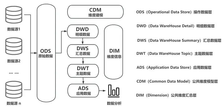
1.1 Typical architecture diagram of traditional data warehouse
The importance of data warehouse lies in its ability to help enterprises achieve centralized management and efficient utilization of data. It can be divided into two types: offline data warehouse and real-time data warehouse according to its purpose and real-time nature.
Offline data warehouses are usually implemented in a T-1 manner, that is, the previous day's historical data is imported into the data warehouse through job tasks at regular times every day (such as in the early morning), and then massive historical data (batch data) are analyzed through OLAP (Online Analytical Processing). Inquire.
For most enterprises, there is an urgent need for T+0 to realize real-time risk control, real-time effect analysis, real-time process control and other functions in business. Traditional offline data warehouses cannot meet real-time requirements, so a new data warehouse architecture that takes into account real-time and analytical capabilities has emerged, that is, real-time data warehouses.
The technical requirements and implementation difficulty of real-time data warehouses far exceed those of traditional data warehouses. Compared with traditional data warehouses, real-time data warehouses can have more efficient data processing capabilities and real-time (quasi-real-time) data update frequency. Under the low-latency performance requirements, technical problems such as data source heterogeneity, data quality control, transactions and strong consistency, multi-mode storage, and high-performance aggregation analysis need to be solved. Moreover, how to enable ordinary developers to have the development and operation and maintenance capabilities of real-time data warehouses, and to continuously and stably carry out product iterations is also a very big test.
1.3 Typical architecture of traditional real-time data warehouse
Traditional real-time data warehouses are usually based on the Hadoop big data framework and use Lambda architecture or Kappa architecture. The technology is complex and the development cycle is long, which is a huge burden for enterprises in terms of developer costs, time costs, and hardware investment costs.
The typical technology stack of traditional real-time data warehouse is as follows:
- Collection (Sqoop, Flume, Flink CDC, DataX, Kafka)
- Storage (HBase, HDFS, Hive, MySQL, MongoDB)
- Data processing and computing (Hive, Spark, Flink, Storm, Presto)
- OLAP analysis and query (TSDB/HTAP, ES, Kylin, DorisDB)
If enterprises want to implement traditional real-time data warehouses, they will face many problems such as high learning costs, large resource consumption, and insufficient scalability and real-time performance.
1.4 DolphinDB real-time data warehouse architecture and performance
Unlike complex traditional real-time data warehouses, DolphinDB can quickly implement lightweight real-time data warehouses through its own product capabilities. It can independently perform collection, storage, flow computing, ETL, decision analysis and calculation, and visual display. It can also be used as an effective supplement to various third-party applications deployed by the enterprise (such as big data platform, AI middle platform, cockpit) to provide real-time data warehouse technical support for enterprise-level application systems and group-level data middle platforms to achieve More complex application scenarios.
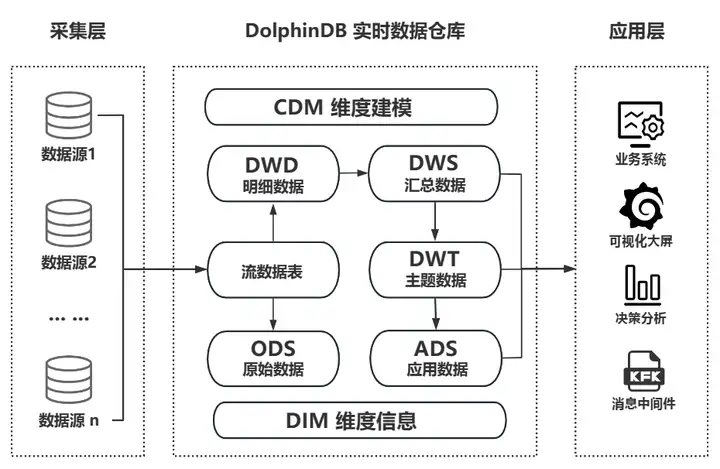
DolphinDB real-time data warehouse business architecture diagram
DolphinDB has rich and mature data warehouse practice cases in various industries such as the Internet of Things and finance, fully demonstrating its extensive application value.
Taking the real-time data warehouse project of a provincial customs electronic port company as an example, the real-time data warehouse built by DolphinDB fully leverages the advantages of All In One's lightweight one-stop product. It supports access to multi-source heterogeneous data, is compatible with standard SQL, supports complex multi-table associations, and has powerful ETL data cleaning capabilities, which greatly shortens the data processing chain and reduces operation, maintenance and development costs. Its business structure and technical characteristics are shown in the figure below:
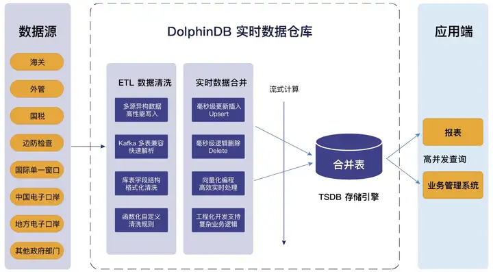
Business structure diagram of a province’s electronic port real-time data warehouse project
The following is a reference for the real-time data warehouse performance indicators that DolphinDB can support when deploying a three-machine high-availability cluster:
- Number of measuring points supported: >100 million measuring points
- Write throughput: >100 million measurement points/second
- Number of records supported by ODS: > 1 trillion
- Maximum number of client connections: >5000
- Concurrent queries (QPS): >5000
- Multi-dimensional aggregation query: millisecond level
- Real-time stream computing feature value extraction: >500,000/second
- Synchronization time for deletion and modification (soft deletion, upsert) of a single record and single process: ≈ 10ms
- High availability cluster: multiple copies (data high availability), multiple control nodes (metadata high availability), client disconnection reconnection and failover (client high availability)
- Elastic expansion: horizontal expansion (adding nodes) without downtime, vertical expansion (adding disk volumes) without downtime, and supports grayscale upgrades
2. DolphinDB real-time data warehouse practice
Next, we will use DolphinDB to build a lightweight real-time data warehouse using the real needs of real-time monitoring of hydropower station generator equipment as an example. This case can be applied to energy and power, industrial Internet of Things, Internet of Vehicles and other industries.
Everyone is welcome to try it and verify it together!
2.1 DolphinDB installation and deployment
1. Download the latest version of the official website community, version 2.00.11 or above is recommended.
Portal: https://cdn.dolphindb.cn/downloads/DolphinDB_Win64_V2.00.11.3.zip
2. There should be no spaces in the windows decompression path to avoid installing it in the Program Files path.
Official website tutorial: https://docs.dolphindb.cn/zh/tutorials/deploy_dolphindb_on_new_server.htm l
3. This test uses the enterprise version, and you can apply for a free trial license. If you use the free community version, it is recommended to reduce the data level of the test.
How to obtain: https://dolphindb.cn/product# downloads
4. If you have any questions during the installation and testing process, you can send a private message in the background for consultation.
2.2 Real-time data warehouse indicator requirements
- Basic data situation
Number of measuring points: 40000
Sampling frequency: seconds
- Calculated indicator (aggregated value)

2.3 Practical plan planning
Based on the DolphinDB stream computing framework, a lightweight real-time data warehouse at the edge is built. All calculation results are completed efficiently while data is written, and the delay is controlled at the millisecond level.
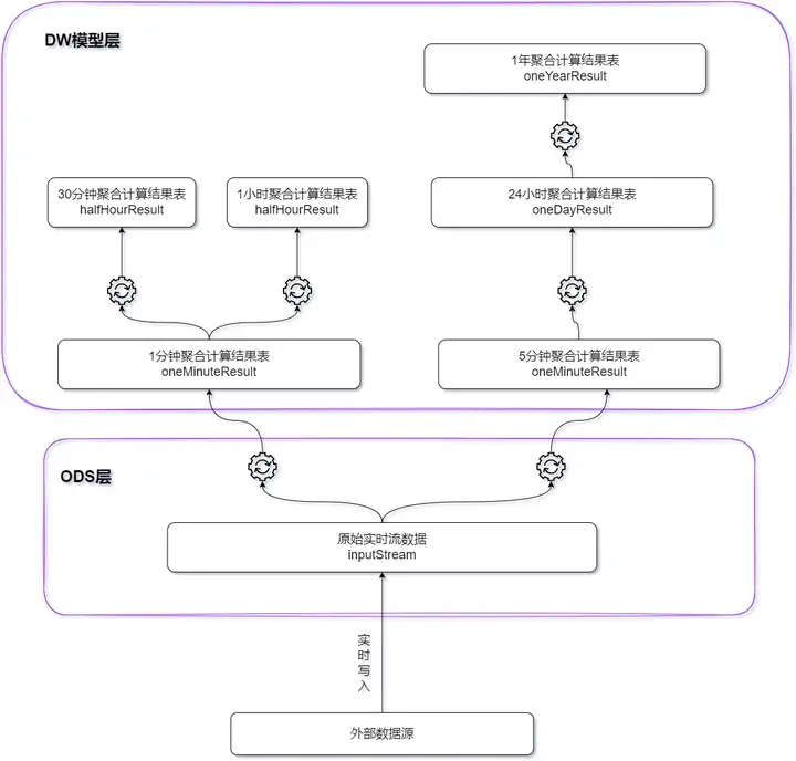
- For indicators with a 1-minute calculation period and a 5-minute calculation period, the original real-time data is used as the base table;
- For indicators with a 30-minute calculation period and a 1-hour calculation period, the 1-minute calculation result is used as the base table;
- For 24-hour calculation cycle indicators, the 5-minute calculation result is used as the base table;
- For indicators with a one-year calculation period, the 24-hour calculation results are used as the base table.
The calculation window and sliding step size of each type of indicator are as shown in the following table:
| Calculation cycle | window length | sliding step size | Remark |
|---|---|---|---|
| 1 minute | 1 minute | 1 minute | Every 1 minute, the values in the past 1 minute window are calculated |
| 5 minutes | 5 minutes | 5 minutes | Every 5 minutes, the values within the past 5 minute window are calculated |
| 30 minutes | 30 minutes | 30 minutes | Every 30 minutes, the values within the past 30 minute window are calculated |
| 1 hour | 1 hour | 1 hour | Every 1 hour, the values within the past 1 hour window are calculated. |
| 24 hours | 24 hours | 24 hours | Every 24 hours, the values within the past 24 hour window are calculated |
| 1 year | 1 year | 24 hours | Every 1 day, the values within the past 1 year window are calculated. |
3. Performance testing and results
3.1 Test environment
In order to facilitate testing and verification, a single-machine and single-node deployment method is used to implement a lightweight real-time data warehouse. The server configuration is as follows:
- CPU: 12 cores
- Memory: 32GB
- Disk: 1.1T HDD 150MB/s
Use the script to simulate the real-time data of all measurement points (40000) within 24 hours (2023.01.01T00:00:00-2023.01.02T00:00:01.000), and perform 1 minute, 5 minutes, 30 minutes, 1 hour, and 24 hours Window aggregation calculations are performed and the calculation results are written to the distributed database. (In a certain window, the number of data items may be smaller than the window length)
For the calculation of the 1-year window, real-time data of the calculation results of the 24-hour window are also simulated, and the results of the simulation are aggregated and calculated in real time.
The detailed test script is included in the attachment at the end of the article.
3.2 Test results
The performance test results are shown in the table below:
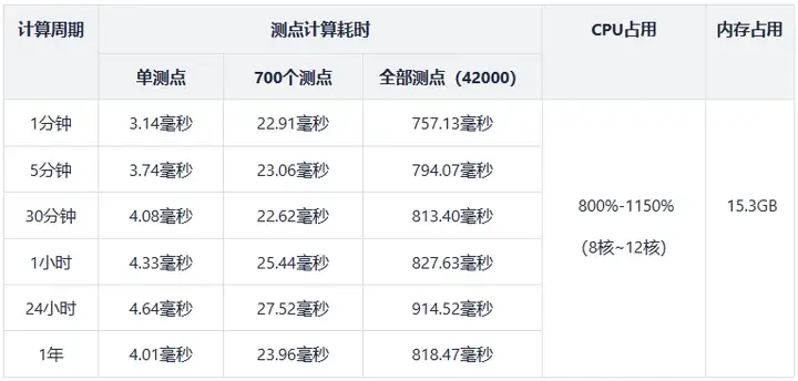
Note: In the above table, the calculation time for all measuring points is the time for calculating the indicators of all measuring points in the time window; the calculation time for single/multiple measuring points is the time for calculating the indicators of the selected measuring points in the time window.
4. Summary
Through the study and practice of this tutorial, we have an in-depth understanding of DolphinDB's powerful capabilities in building lightweight real-time data warehouses. With its high-performance, distributed, and real-time computing characteristics, DolphinDB provides various industries with a powerful tool for quickly realizing low-latency calculation and analysis of complex indicators on massive data.
Through practical operations, we can experience the ease of use and efficiency of DolphinDB. Whether it is data import, data query or complex streaming calculations, DolphinDB provides concise and clear syntax and powerful functions. The script provided in the attachment not only includes the basic usage and operation methods of DolphinDB, but also provides an in-depth understanding of the construction principles and application scenarios of the real-time data warehouse. This allows us to quickly build a real-time data warehouse that meets business needs and respond to various complex analysis needs in real time.
Finally, I hope readers can combine the sample code in this tutorial with their own business characteristics to build a lightweight and high-performance real-time data warehouse. In practical applications, the potential of DolphinDB is continuously explored. Whether it is energy and power, petrochemical industry, intelligent manufacturing, aerospace, Internet of Vehicles, finance and other industries, DolphinDB can provide strong support for a wide range of applications in real-time data warehouses.
5. Accessories
The test results can be reproduced on the DolphinDB server through the following script:
def clearEnv(){
    //取消订阅
    unsubscribeTable(tableName=`inputStream, actionName="dispatch1")
    unsubscribeTable(tableName=`inputStream, actionName="dispatch2")
    unsubscribeTable(tableName=`oneMinuteResult, actionName="calcHalfHour")
    unsubscribeTable(tableName=`oneMinuteResult, actionName="calcOneHour")
    unsubscribeTable(tableName=`fiveMinuteResult, actionName="calcOneDay")
    unsubscribeTable(tableName = `oneDayResultSimulate,actionName=`calcOneYear)

    unsubscribeTable(tableName = `oneMinuteResult,actionName=`appendInToDFS)
    unsubscribeTable(tableName = `fiveMinuteResult,actionName=`appendInToDFS)
    unsubscribeTable(tableName = `halfHourResult,actionName=`appendInToDFS)
    unsubscribeTable(tableName = `oneHourResult,actionName=`appendInToDFS)
    unsubscribeTable(tableName = `oneDayResult,actionName=`appendInToDFS)
    unsubscribeTable(tableName = `oneYearResult,actionName=`appendInToDFS)

    //删除流计算引擎
    for(i in 1..2){
        try{dropStreamEngine(`dispatchDemo+string(i))}catch(ex){print(ex)}
    }
    for(i in 1..5){
        try{dropStreamEngine(`oneMinuteCalc+string(i))}catch(ex){print(ex)}
        try{dropStreamEngine(`fiveMinuteCalc+string(i))}catch(ex){print(ex)}
    }
    try{dropStreamEngine(`halfHourCalc)}catch(ex){print(ex)}
    try{dropStreamEngine(`oneHourCalc)}catch(ex){print(ex)}
    try{dropStreamEngine(`oneDayCalc)}catch(ex){print(ex)}
    try{dropStreamEngine(`oneYearCalc)}catch(ex){print(ex)}

    //删除流数据表
    try{dropStreamTable(`inputStream)}catch(ex){print(ex)}
    try{dropStreamTable(`oneMinuteResult)}catch(ex){print(ex)}
    try{dropStreamTable(`fiveMinuteResult)}catch(ex){print(ex)}
    try{dropStreamTable(`halfHourResult)}catch(ex){print(ex)}
    try{dropStreamTable(`oneHourResult)}catch(ex){print(ex)}
    try{dropStreamTable(`oneDayResult)}catch(ex){print(ex)}
    try{dropStreamTable(`oneDayResultSimulate)}catch(ex){print(ex)}
    try{dropStreamTable(`oneYearResult)}catch(ex){print(ex)}

}

def createStreamTable(){
    //定义输入流表
    enableTableShareAndPersistence(table = streamTable(1000:0,`Time`deviceId`value,`TIMESTAMP`SYMBOL`DOUBLE),
            tableName = `inputStream,cacheSize = 1000000,precache=1000000)

    colName = `Time`deviceId`filterTime`MAX`MIN`MEAN`MED`P95`P5`CHANGE`CHANGE_RATE`first`last`endTime
    colType = `TIMESTAMP`SYMBOL`NANOTIMESTAMP join take(`DOUBLE,10) join `NANOTIMESTAMP
    //定义1分钟窗口计算结果流表
    enableTableShareAndPersistence(table = streamTable(1000:0,colName,colType),
        tableName = `oneMinuteResult,cacheSize = 1000000,precache=1000000)

    //定义5分钟窗口计算结果流表
    enableTableShareAndPersistence(table = streamTable(1000:0,colName,colType),
        tableName = `fiveMinuteResult,cacheSize = 1000000,precache=1000000)

    //定义30分钟窗口计算结果流表
    enableTableShareAndPersistence(table = streamTable(1000:0,colName,colType),
        tableName = `halfHourResult,cacheSize = 1000000,precache=1000000)

    //定义1小时窗口计算结果流表
    enableTableShareAndPersistence(table = streamTable(1000:0,colName,colType),
        tableName = `oneHourResult,cacheSize = 1000000,precache=1000000)

    //定义24小时窗口计算结果流表
    enableTableShareAndPersistence(table = streamTable(1000:0,colName,colType),
        tableName = `oneDayResult,cacheSize = 1000000,precache=1000000)

    //定义模拟24小时窗口计算结果流表
    colName = `TIME`deviceId`MAX`MIN`MEAN`MED`P95`P5`CHANGE`CHANGE_RATE`first`last
    colType = `DATE`SYMBOL join take(`DOUBLE,10)
    enableTableShareAndPersistence(table = streamTable(1000:0,colName,colType),
        tableName = `oneDayResultSimulate,cacheSize = 1000000,precache=1000000)

    //定义1年窗口计算结果流表
    colName = `Time`deviceId`filterTime`MAX`MIN`MEAN`MED`P95`P5`CHANGE`CHANGE_RATE`first`last`endTime
    colType = `DATE`SYMBOL`NANOTIMESTAMP join take(`DOUBLE,10) join `NANOTIMESTAMP
    enableTableShareAndPersistence(table = streamTable(1000:0,colName,colType),
       tableName = `oneYearResult,cacheSize = 1000000,precache=1000000)
}

def createDFS(){
    //创建存储计算1分钟窗口计算结果表
    if(existsDatabase("dfs://oneMinuteCalc")){dropDatabase("dfs://oneMinuteCalc")}
    db1 = database(, VALUE,2023.01.01..2023.01.03)
    db2 = database(, HASH,[SYMBOL,20])
    db = database(directory="dfs://oneMinuteCalc", partitionType=COMPO, partitionScheme=[db1,db2],engine="TSDB")
    colName =  `Time`deviceId`filterTime`MAX`MIN`MEAN`MED`P95`P5`CHANGE`CHANGE_RATE`first`last`endTime
    colType = `TIMESTAMP`SYMBOL`NANOTIMESTAMP join take(`DOUBLE,10) join `NANOTIMESTAMP
    t = table(1:0,colName,colType)
    pt = db.createPartitionedTable(table=t,tableName ="test" ,partitionColumns = ["Time","deviceId"],
            sortColumns =["deviceId","Time"],compressMethods={Time:"delta"})

    //创建存储计算5分钟窗口计算结果表
    if(existsDatabase("dfs://fiveMinuteCalc")){dropDatabase("dfs://fiveMinuteCalc")}
    db = database(directory="dfs://fiveMinuteCalc", partitionType=VALUE,
           partitionScheme=2023.01.01..2023.01.03,engine="TSDB")
    t = table(1:0,colName,colType)
    pt = db.createPartitionedTable(table=t,tableName ="test" ,partitionColumns = ["Time"],
            sortColumns =["deviceId","Time"],compressMethods={Time:"delta"},
            sortKeyMappingFunction=[hashBucket{,100}])

    //创建存储计算30分钟窗口计算结果表
    if(existsDatabase("dfs://halfHourCalc")){dropDatabase("dfs://halfHourCalc")}
    db = database(directory="dfs://halfHourCalc", partitionType=VALUE,
            partitionScheme=2023.01.01..2023.01.03,engine="TSDB")
    t = table(1:0,colName,colType)
    pt = db.createPartitionedTable(table=t,tableName ="test" ,partitionColumns = ["Time"],
            sortColumns =["deviceId","Time"],compressMethods={Time:"delta"})

    //创建存储计算1小时窗口计算结果表
    if(existsDatabase("dfs://oneHourCalc")){dropDatabase("dfs://oneHourCalc")}
    db = database(directory="dfs://oneHourCalc", partitionType=VALUE,
             partitionScheme=2023.01.01..2023.01.03,engine="TSDB")
    t = table(1:0,colName,colType)
    pt = db.createPartitionedTable(table=t,tableName ="test" ,partitionColumns = ["Time"],
            sortColumns =["deviceId","Time"],compressMethods={Time:"delta"})

    //创建存储计算24小时窗口计算结果表
    if(existsDatabase("dfs://oneDayCalc")){dropDatabase("dfs://oneDayCalc")}
    db = database(directory="dfs://oneDayCalc", partitionType=VALUE,
          partitionScheme=2023.01.01..2023.01.03,engine="TSDB")
    t = table(1:0,colName,colType)
    pt = db.createPartitionedTable(table=t,tableName ="test" ,partitionColumns = ["Time"],
            sortColumns =["deviceId","Time"],compressMethods={Time:"delta"})

    //创建存储计算1年窗口计算结果表
    if(existsDatabase("dfs://oneYearCalc")){dropDatabase("dfs://oneYearCalc")}
    db = database(directory="dfs://oneYearCalc", partitionType=VALUE,
          partitionScheme=2023.01.01..2023.01.03,engine="TSDB")
    t = table(1:0,colName,colType)
    pt = db.createPartitionedTable(table=t,tableName ="test" ,partitionColumns = ["Time"],
            sortColumns =["deviceId","Time"],compressMethods={Time:"delta"})
}

//1分钟窗口计算过滤函数
def filter1(msg){
    t = select *,now(true) as filterTime from msg
    getStreamEngine(`dispatchDemo1).append!(t)
}

//5分钟窗口计算过滤函数
def filter2(msg){
    t = select *,now(true) as filterTime from msg
    getStreamEngine(`dispatchDemo2).append!(t)
}

//30分钟窗口计算过滤函数
def filter3(msg){
    t = select *,now(true) as filterTime2 from msg
    getStreamEngine(`halfHourCalc).append!(t)
}

//1小时窗口计算
def filter4(msg){
    t = select *,now(true) as filterTime2 from msg
    getStreamEngine(`oneHourCalc).append!(t)
}

//24小时窗口计算
def filter5(msg){
    t = select *,now(true) as filterTime2 from msg
    getStreamEngine(`oneDayCalc).append!(t)
}

clearEnv();
createStreamTable();
createDFS();

schemas1 = table(1:0,`Time`deviceId`value`filterTime,`TIMESTAMP`SYMBOL`DOUBLE`NANOTIMESTAMP)
metrics1 = <[first(filterTime),max(value),min(value),mean(value),med(value),percentile(value,95),
              percentile(value,5),last(value)-first(value),
              (last(value)-first(value))/first(value),first(value),last(value),now(true)]>
//创建1分钟窗口聚合计算引擎
for(i in 1..5){
    engine1 = createTimeSeriesEngine(name="oneMinuteCalc"+string(i), windowSize=60000, step=60000,
                metrics=metrics1 , dummyTable=schemas1 , outputTable=objByName(`oneMinuteResult),
                timeColumn = `Time, useSystemTime=false, keyColumn = `deviceId)
}

//创建5分钟窗口聚合计算引擎
for(i in 1..5){
    engine2 = createTimeSeriesEngine(name="fiveMinuteCalc"+string(i), windowSize=300000, step=300000,
                metrics=metrics1 , dummyTable=schemas1 , outputTable=objByName(`fiveMinuteResult),
                timeColumn = `Time, useSystemTime=false, keyColumn = `deviceId)
}

//1分钟、5分钟窗口聚合计算分发引擎
dispatchEngine1=createStreamDispatchEngine(name="dispatchDemo1", dummyTable=schemas1, keyColumn=`deviceId,
        outputTable=[getStreamEngine("oneMinuteCalc1"),getStreamEngine("oneMinuteCalc2"),
                        getStreamEngine("oneMinuteCalc3"),getStreamEngine("oneMinuteCalc4"),
                        getStreamEngine("oneMinuteCalc5")])
dispatchEngine2=createStreamDispatchEngine(name="dispatchDemo2", dummyTable=schemas1, keyColumn=`deviceId,
        outputTable=[getStreamEngine("fiveMinuteCalc1"),getStreamEngine("fiveMinuteCalc2"),
                        getStreamEngine("fiveMinuteCalc3"),getStreamEngine("fiveMinuteCalc4"),
                        getStreamEngine("fiveMinuteCalc5")])


colName =  `Time`deviceId`filterTime`MAX`MIN`MEAN`MED`P95`P5`CHANGE`CHANGE_RATE`first`last`endTime`filterTime2
colType = `TIMESTAMP`SYMBOL`NANOTIMESTAMP join take(`DOUBLE,10) join `NANOTIMESTAMP`NANOTIMESTAMP
schemas2 = table(1:0,colName,colType)
metrics2 = <[first(filterTime2),max(MAX),min(MIN),mean(MEAN),med(MED),avg(P95),avg(P5),last(last)-first(first),
                (last(last)-first(first))/first(first),first(first),last(last),now(true)]>
//创建30分钟窗口聚合计算引擎
engine3 = createTimeSeriesEngine(name="halfHourCalc", windowSize=1800000, step=1800000, metrics=metrics2 ,
                dummyTable=schemas2 , outputTable=objByName(`halfHourResult),
                timeColumn = `Time, useSystemTime=false, keyColumn = `deviceId)

//创建1小时窗口聚合计算引擎
engine4 = createTimeSeriesEngine(name="oneHourCalc", windowSize=3600000, step=3600000, metrics=metrics2 ,
                dummyTable=schemas2 , outputTable=objByName(`oneHourResult),
                timeColumn = `Time, useSystemTime=false, keyColumn = `deviceId)

//创建24小时窗口聚合计算引擎
engine5 = createTimeSeriesEngine(name="oneDayCalc", windowSize=86400000, step=86400000,
                metrics=metrics2 , dummyTable=schemas2 , outputTable=objByName(`oneDayResult),
                timeColumn = `Time, useSystemTime=false, keyColumn = `deviceId)


//订阅
subscribeTable(tableName=`inputStream, actionName="dispatch1", handler=filter1, msgAsTable = true,
          batchSize = 10240)
subscribeTable(tableName=`inputStream, actionName="dispatch2", handler=filter2, msgAsTable = true,
          batchSize = 10240)

subscribeTable(tableName=`oneMinuteResult, actionName="calcHalfHour", handler=filter3,
           msgAsTable = true,batchSize = 10240)
subscribeTable(tableName=`oneMinuteResult, actionName="calcOneHour", handler=filter4,
          msgAsTable = true,batchSize = 10240)
subscribeTable(tableName=`fiveMinuteResult, actionName="calcOneDay", handler=filter5,
          msgAsTable = true,batchSize = 10240)


subscribeTable(tableName = `oneMinuteResult,actionName=`appendInToDFS,offset=0,
          handler=loadTable("dfs://oneMinuteCalc","test"),
          msgAsTable=true,batchSize=10240)
subscribeTable(tableName = `fiveMinuteResult,actionName=`appendInToDFS,offset=0,
          handler=loadTable("dfs://fiveMinuteCalc","test"),
          msgAsTable=true,batchSize=10240)
subscribeTable(tableName = `halfHourResult,actionName=`appendInToDFS,offset=0,
          handler=loadTable("dfs://halfHourCalc","test"),
          msgAsTable=true,batchSize=10240)
subscribeTable(tableName = `oneHourResult,actionName=`appendInToDFS,offset=0,
          handler=loadTable("dfs://oneHourCalc","test"),
          msgAsTable=true,batchSize=10240)
subscribeTable(tableName = `oneDayResult,actionName=`appendInToDFS,offset=0,
          handler=loadTable("dfs://oneDayCalc","test"),
          msgAsTable=true,batchSize=10240)


def filter6(msg){
    tmp = select * ,now(true) as filterTime from msg
    getStreamEngine(`oneYearCalc).append!(tmp)
}

colName =  `Time`deviceId`MAX`MIN`MEAN`MED`P95`P5`CHANGE`CHANGE_RATE`first`last`filterTime
colType = `DATE`SYMBOL join take(`DOUBLE,10) join `NANOTIMESTAMP
schemas3 = table(1:0,colName,colType)
metrics3 = <[last(filterTime),max(MAX),min(MIN),mean(MEAN),med(MED),avg(P95),avg(P5),last(last)-first(first),
                (last(last)-first(first))/first(first),first(first),last(last),now(true)]>
engine6 = createTimeSeriesEngine(name="oneYearCalc", windowSize=365, step=1, metrics=metrics3 ,
            dummyTable=schemas3 , outputTable=objByName(`oneYearResult),
            timeColumn = `Time, useSystemTime=false, keyColumn = `deviceId)

subscribeTable(tableName = `oneDayResultSimulate,actionName=`calcOneYear, handler=filter6,
            msgAsTable = true,batchSize = 10240)
subscribeTable(tableName = `oneYearResult,actionName=`appendInToDFS,offset=0,
            handler=loadTable("dfs://oneYearCalc","test"),
            msgAsTable=true)


deviceIdList = lapd(string(rand(10000,700)),6,"0")  //测点id

//模拟数据的函数,一共模拟1小时的数据
def simulateData(deviceIdList){
    num = deviceIdList.size()
    startTime = timestamp(2023.01.01)
    do{
        Time = take(startTime,num)
        deviceId = deviceIdList
        value = rand(100.0,num)
        objByName(`inputStream).append!(table(Time,deviceId,value))
        startTime = startTime+1000
        sleep(100)
    }while(startTime<=2023.01.02T00:00:10.000)
}

def simulateOneDay(deviceIdList){
    num = deviceIdList.size()
    startTime =2022.01.01
    do{
        Time = take(startTime,num)
        deviceId = deviceIdList
        MAX = rand(100.0,num)
        MIN = rand(100.0,num)
        MEAN = rand(100.0,num)
        MED = rand(100.0,num)
        P95 = rand(100.0,num)
        P5 = rand(100.0,num)
        CHANGE = rand(100.0,num)
        CHANGE_RATE = rand(100.0,num)
        first = rand(100.0,num)
        last = rand(100.0,num)
        tmp = table(Time,deviceId,MAX,MIN,MEAN,MED,P95,P5,CHANGE,CHANGE_RATE,first,last)
        objByName(`oneDayResultSimulate).append!(tmp)
        startTime = startTime+1
        sleep(500)
    }while(startTime<=2023.12.31)
}


submitJob("simulateData","write",simulateData,deviceIdList)
submitJob("simulateOneDay","write",simulateOneDay,deviceIdList)


//耗时统计
tmp1 = select Time,deviceId,filterTime,endTime from loadTable("dfs://oneYearCalc","test") order by Time,deviceId
tmp2 = select Time,deviceId,next(filterTime) as startTime,endTime from tmp1 context by deviceId
select avg(endTime-startTime)\1000\1000 as timeUsed from tmp2 group by deviceId  //统计单个测点的计算耗时
tmp3 = select min(startTime) as st,max(endTime) as dt from tmp2 group by Time
select (dt-st)\1000\1000 as used from tmp3 //统计整个时间窗口的计算耗时