Andrew Ng's "Machine Learning" - Linear Regression Code Implementation

Data sets and source files can be obtained in the Github project

Address: https://github.com/Raymond-Yang-2001/AndrewNg-Machine-Learing-Homework

1. Univariate linear regression

Univariate linear regression finds a one-dimensional equation and fits a straight line.

Univariate linear regression formula

$$h_{w,b}(x)=b+wx$$
$w$ and$b$ is a parameter. To facilitate calculation, you can give$x$ plus an$x_0=1$
$$h_{w,b}\left(x\right)=b{x}_0+w{x}_1$$

loss function

$$J(w,b)=\frac{1}{2m\_}\sum _{i=1}^m(h_{w,b}(x^{(i)})-y^{\left(i\right)}{)}^2$$
In order to avoid excessive or small losses caused by inappropriate data ranges (for example, if the data value is too large, the loss may be$10^5$ or$10^6$ , this order of magnitude is not suitable for intuitive analysis) When evaluating the loss, you can hw$h_{w,b}\left(x^{\left(i\right)}\right)$sumy$y^{\left(i\right)}$ First standardize so that the loss value is within an evaluable range. But this is not done when doing gradient descent

Optimization Algorithm—Batch Gradient Descent (BGD)

$$w_j=w_j-a\frac{\partial }{\partial w_j}J(w,b)=w_j-a\frac{1}{m}\sum _{i=1}^m\left(h_{w,b}\right(x^{\left(i\right)})-y^{(i)})x^{(i)}$$
$$b_j=b_j-a\frac{\partial }{\partial b_j}J(w,b)=w_j-a\frac{1}{m}\sum _{i=1}^m\left(h_{w,b}\right(x^{\left(i\right)})-y^{\left(i\right)})$$
Here, we can use$\theta$ unified identification parameters, including$w$ and$b$。

That is, $j$ parameters$i_j$Determine the following:
$$i_j=i_j-a\frac{\partial }{\partial w_j}J(\theta ;\mathbf{x})=w_j-a\frac{1}{m}\sum _{i=1}^m\left(h_{}\right(x^{\left(i\right)})-y^{\left(i\right)})x^{\left(i\right)}$$
where$\alpha$ is the learning rate.

2. Multivariable linear regression

Multivariable linear regression attempts to find the relationship between multiple variables and predicted values. For example, the relationship between house size, number of bedrooms in a house, and house prices.

Feature scaling (normalization)

When the numerical differences between different features of the sample are too large, gradient-based optimization methods will have some problems. For example, there is the following regression equation:
$$h_{}(x)=i_0+i_1{x}_1+i_2{x}_2$$
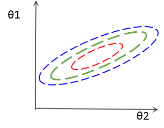
Assume $x_2$The range is $0\sim 1$，$x_1$The range is $10^3\sim 10^4$ . We simultaneously optimize$i_0\sim i_2$, so that they all change by the same size, then obviously when the input samples are the same, $i_1$The change will be greater than $i_2$changes that lead to greater output. This can also be understood as the model pair $i_1$More sensitive. As shown in the following loss isoline diagram, $i_1$Small changes can bring drastic changes in losses. In this case, parameter optimization will be more difficult.

One way to solve this problem is feature scaling, which scales two features to the same range. For example, z-score normalization can be performed:
$$x_{new}=\frac{x-}{p}$$
Among them, $\mu$ is the mean of the data set,$\sigma$ is the standard deviation, and the distribution of new data is a distribution with mean 0 and standard deviation 1.
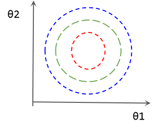
The parameter loss diagram after data normalization is as follows:

Inverse scaling of parameters

Since the data is scaled, the final parameters will also be scaled accordingly. The specific relationship is as follows:
$$i_0+i_{1\sim d+1}\frac{x_{1\sim d+1}-m_x}{p_x}=\frac{y-m_y}{p_y}$$
Here we are talking about $y$ has also been standardized.In fact, it is not necessary to do this, and there will be no impact on performance. But the normalization of y makes the parameters smaller, and convergence can be achieved faster for parameters initialized to 0.

In $In$ this case, the inverse scaling formula of the parameters is:
$$i_{1\sim d+1}^{new}=\frac{i_{1\sim d+1}}{p_x}{p}_y$$
Formula:
$$i_0{p}_y+i_{1\sim d+1}^{new}(x_{1\sim d+1}-m_x)=y-m_y$$

$$i_0^{new}=i_0{p}_y+m_y-i_{1\sim d+1}^{new}{m}_x$$
Among them, during vectorization operation, $i_{1\sim d+1}^{new}$和$m_x$They are all vectors of (1,d), and multiplication should use vector inner product.

3. Linear regression algorithm code implementation

vector implementation

Let the data $The\; dimensions\; of\; x$ are$(n,d)$ , where n is the number of samples and d is the dimension of the sample features. For the convenience of calculation, we add an extra feature dimension with all values ​​​​1 to the sample, so that its dimension becomes$(n,d+1)$

1. Prediction
   Let the parameter $The\; dimension\; of\; \theta$ is (1, d+1), then$\mathbf{x}{\mathbf{\theta }}^{\top }$或$(\mathbf{\theta }{\mathbf{x}}^{\top }{)}^{\top The}$ dimension can be obtained as$(n,1)$ Prediction result$h_{}(\mathbf{x})$。
2. Let us divide the
   quantity j by the quantity:
   $$i_j=i_j-a\frac{\partial }{\partial w_j}J(\theta ;\mathbf{x})=w_j-a\frac{1}{m}\sum _{i=1}^m(h_{}(x^{(i)})-y^{(i)})x^{\left(i\right)}$$
   In fact, here we put$i_0$As a bias, its gradient should be:
   $$\frac{\partial }{\partial w_0}J(\theta ;x)=w_0-a\frac{1}{m}\sum _{i=1}^m\left(h_{}\right(x^{\left(i\right)})-y^{\left(i\right)})$$, since we supplement the data with feature dimensions$x_0$, so it can be calculated using the above formula like other parameters.
   Let $error$ matrix$\mathbf{\beta }$为$h_{}(\mathbf{x})-x$ , with dimensions$(n,1)$ , then$x^{\top }\beta /n$is the dimension$(d+1,1)$的梯度矩阵。
   $$x^{\top }\mathbf{\beta }=\left[\begin{array}{ccc}{x}^{(1)}& x^{(2)}& \cdots \end{array}\right]\times \left[\begin{array}{c}h(x^{(1)})-y^{(1)}\\ h(x^{(2)})-y^{(2)}\\ ⋮\end{array}\right]=\left[\begin{array}{c}{\sum }_{i=1}^n(h(x^{(i)})-y^{(i)})x_0^{(1)}\\ {\sum }_{i=1}^n\left(h\right(x^{\left(i\right)})-y^{\left(i\right)})x_1^{\left(1\right)}\\ ⋮\end{array}\right]$$
   ${\mathbf{x}}^{}$Each element in${}^{\top }$$\beta$$/$$n$

Python code

import numpy as np


def square_loss(pred, target):
    """
    计算平方误差
    :param pred: 预测
    :param target: ground truth
    :return: 损失序列
    """
    return np.sum(np.power((pred - target), 2))


def compute_loss(pred, target):
    """
    计算归一化平均损失
    :param pred: 预测
    :param target: ground truth
    :return: 损失
    """
    pred = (pred - pred.mean(axis=0)) / pred.std(axis=0)
    target = (pred - target.mean(axis=0)) / target.std(axis=0)
    loss = square_loss(pred, target)
    return np.sum(loss) / (2 * pred.shape[0])


class LinearRegression:
    """
    线性回归类
    """

    def __init__(self, x, y, val_x, val_y, epoch=100, lr=0.1):
        """
        初始化
        :param x: 样本, (sample_number, dimension)
        :param y: 标签, (sample_numer, 1)
        :param epoch: 训练迭代次数
        :param lr: 学习率
        """
        self.theta = None
        self.loss = []
        self.val_loss = []
        self.n = x.shape[0]
        self.d = x.shape[1]

        self.epoch = epoch
        self.lr = lr

        t = np.ones(shape=(self.n, 1))

        self.x_std = x.std(axis=0)
        self.x_mean = x.mean(axis=0)
        self.y_mean = y.mean(axis=0)
        self.y_std = y.std(axis=0)

        x_norm = (x - self.x_mean) / self.x_std
        y_norm = (y - self.y_mean) / self.y_std

        self.y = y_norm
        self.x = np.concatenate((t, x_norm), axis=1)

        self.val_x = val_x
        self.val_y = val_y

    def init_theta(self):
        """
        初始化参数
        :return: theta (1, d+1)
        """
        self.theta = np.zeros(shape=(1, self.d + 1))

    def validation(self, x, y):
        x = (x - x.mean(axis=0)) / x.std(axis=0)
        y = (y - y.mean(axis=0)) / y.std(axis=0)
        outputs = self.predict(x)
        curr_loss = square_loss(outputs, y) / (2 * y.shape[0])
        return curr_loss

    def gradient_decent(self, pred):
        """
        实现梯度下降求解
        """
        # error (n,1)
        error = pred - self.y
        # gradient (d+1, 1)
        gradient = np.matmul(self.x.T, error)
        # gradient (1,d+1)
        gradient = gradient.T / pred.shape[0]
        # update parameters
        self.theta = self.theta - (self.lr / self.n) * gradient

    def train(self):
        """
        训练线性回归
        :return: 参数矩阵theta (1,d+1); 损失序列 loss
        """
        self.init_theta()

        for i in range(self.epoch):
            # pred (1,n); theta (1,d+1); self.x.T (d+1, n)
            pred = np.matmul(self.theta, self.x.T)
            # pred (n,1)
            pred = pred.T
            curr_loss = square_loss(pred, self.y) / (2 * self.n)
            val_loss = self.validation(self.val_x, self.val_y)
            self.gradient_decent(pred)
            
            self.val_loss.append(val_loss)
            self.loss.append(curr_loss)
            print("Epoch: {}/{}\tTrain Loss: {:.4f}\tVal loss: {:.4f}".format(i + 1, self.epoch, curr_loss, val_loss))

        # un_scaling parameters
        self.theta[0, 1:] = self.theta[0, 1:] / self.x_std.T * self.y_std[0]
        self.theta[0, 0] = self.theta[0, 0] * self.y_std[0] + self.y_mean[0] - np.dot(self.theta[0, 1:], self.x_mean)
        return self.theta, self.loss, self.val_loss

    def predict(self, x):
        """
        回归预测
        :param x: 输入样本 (n,d)
        :return: 预测结果 (n,1)
        """
        # (d,1)
        t = np.ones(shape=(x.shape[0], 1))
        x = np.concatenate((t, x), axis=1)
        pred = np.matmul(self.theta, x.T)
        return pred.T

4. Experimental results

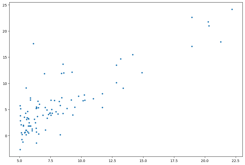
Univariate regression

Data set visualization

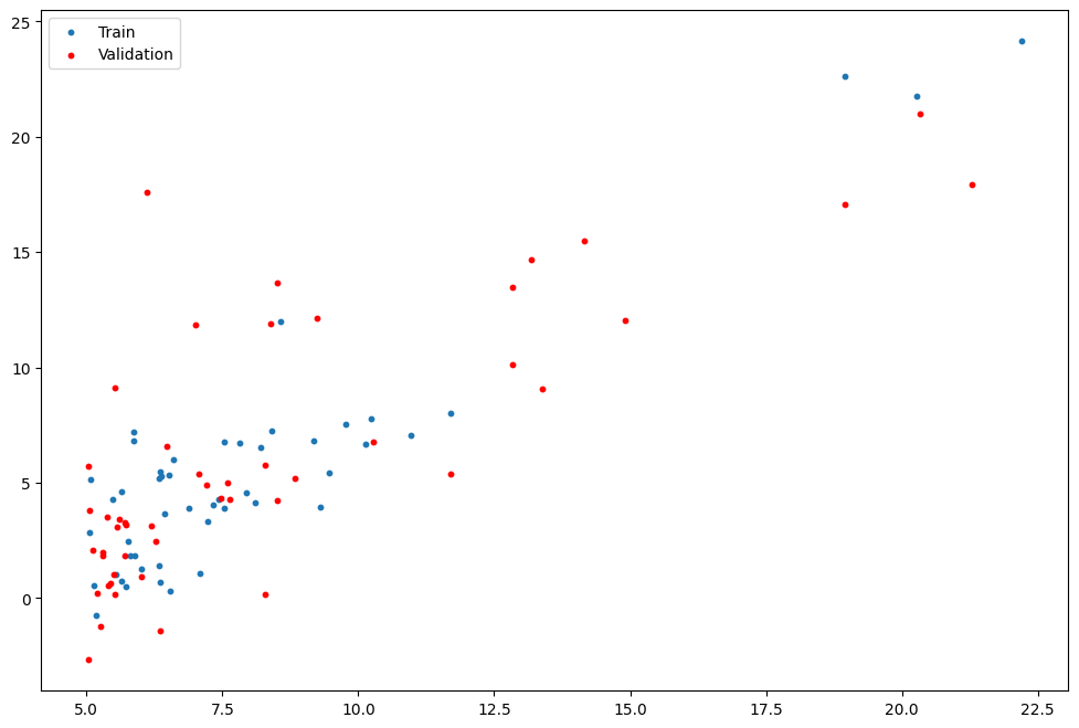
training set and test set division

from LinearRegression import LinearRegression

epochs = 200
alpha = 1
linear_reg = LinearRegression(x=train_x_ex,y=train_y_ex,val_x=val_x_ex, val_y=val_y_ex, lr=alpha,epoch=epochs)
start_time = time.time()
theta,loss, val_loss = linear_reg.train()
end_time = time.time()

Train Time: 0.0309s
Val Loss: 6.7951

Training process visualization

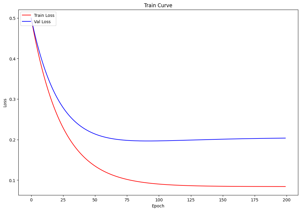
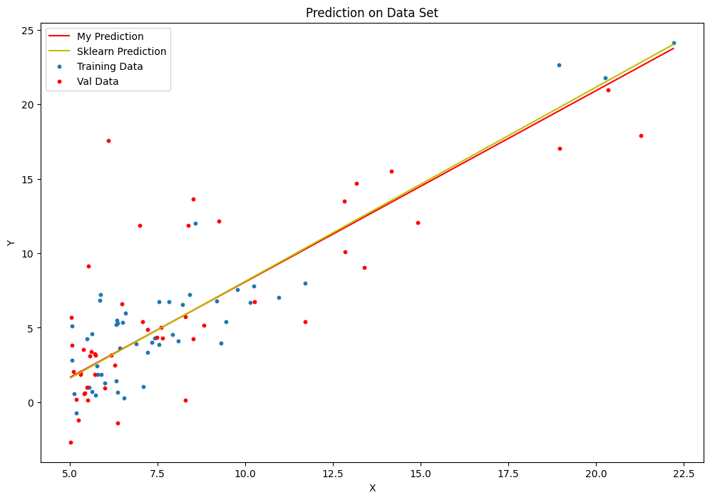
and sk-learn comparison prediction curve

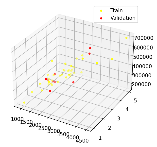
multivariable regression

Data visualization and training set and validation set

from LinearRegression import LinearRegression

alpha = 0.1
epochs = 1000
multi_lr = LinearRegression(train_x,train_y_ex,val_x=val_x,val_y=val_y_ex, epoch=epochs,lr=alpha)
start_time = time.time()
theta, loss, val_loss = multi_lr.train()
end_time = time.time()

Train Time: 0.1209s
Val Loss: 4.187（采用归一化后数据计算损失）

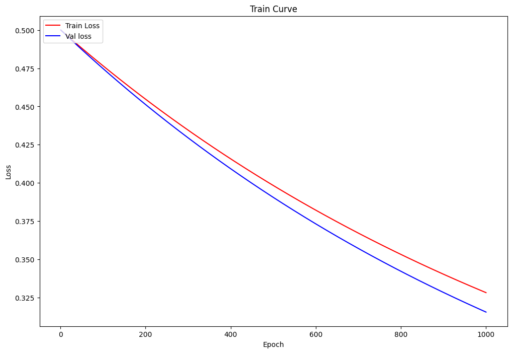
Visualization of the training process

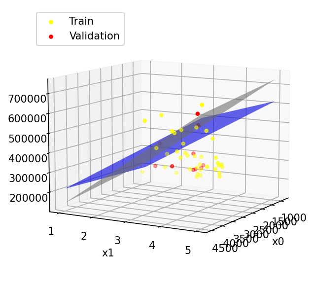
Prediction plane (compared with sk-learn)
where blue is the prediction plane of this algorithm and gray is the prediction plane of sk-learn

Experiment summary

For the implementation of linear regression algorithm to achieve better performance, you can try to adjust the learning rate or the number of iterations to obtain better performance. Since matrix operations are used instead of loops, the training time is greatly shortened, but it has not yet reached the level of the sk-learn library function.