1.Channel exchange
reads the image, and then replaces the RGB channel with the BGR channel. It should be noted that the image read by opencv is BGR by default. cv2.cvtColor function can refer toColor Space Conversions
img = cv2.imread('imori.jpg')
img = cv2.cvtColor(img, cv2.COLOR_BGR2RGB)
cv2.imwrite('answer.png', img)
2.Grayscale
The calculation formula for grayscale is:
![]()
img = cv2.cvtColor(img, cv2.COLOR_BGR2GRAY)3. Thresholding
Set the pixel value greater than the threshold to 255, otherwise set it to 0. For the cv2.threshold function, please refer toMiscellaneous Image Transformations
img = cv2.cvtColor(img, cv2.COLOR_BGR2GRAY)
ret, img = cv2.threshold(img, 128, 255, cv2.THRESH_BINARY)
4. Otsu's method
Otsu's algorithm is an algorithm that can automatically determine the threshold value in binarization. https://docs.opencv.org/master/d7/d4d/tutorial_py_thresholding.html The "Otsu"s Binarization" chapter of this page
img = cv2.cvtColor(img, cv2.COLOR_BGR2GRAY)
ret, img = cv2.threshold(img, 0, 255, cv2.THRESH_BINARY+cv2.THRESH_OTSU)
5. HSV transformation
Inverts the hue of an image represented using HSV. Note that Hue represents color from 0° to 360°. HSV color model can refer tohttps://baike.baidu.com/item/HSV/547122
img = cv2.cvtColor(img, cv2.COLOR_BGR2HSV)
# 进行色相反转
img[:, :, 0] = (img[:, :, 0] + 180) % 360
img = cv2.cvtColor(img, cv2.COLOR_HSV2BGR)
6. Subtractive color processing
Compress the image value from 2563 to 43, that is, the RGB value only takes {32,96,169,224}
img = img // 64 * 64 + 327. Average Pooling
Divide the image into fixed-size grids, and the pixel value in the grid is the average of all pixels in the grid. It seems that the operation of pooling is not found in opencv, only the implementation in skimage https://stackoverflow.com/questions/42463172/how-to-perform-max-mean -pooling-on-a-2d-array-using-numpy
img = skimage.measure.block_reduce(img, (8, 8, 1), np.mean)8. Max Pooling
Similar to average pooling
img = skimage.measure.block_reduce(img, (8, 8, 1), np.max)9. Gaussian Filter
Use Gaussian filter (3×3 size, standard deviation �=1.3) for noise reduction. The Gaussian filter smoothes the center pixel according to the weighted average of the Gaussian distribution. For cv2.GaussianBlur function, please refer to OpenCV: Image Filtering. The 8-neighboring Gaussian filter with standard deviation �=1.3 is:

img = cv2.GaussianBlur(img, (3, 3), 1.3)10. Median Filter
Use median filter (3×3 size) for noise reduction. cv2.medianBlur function can refer toOpenCV: Image Filtering
img = cv2.medianBlur(img, 3)11. Mean filter
Use the mean filter (3×3 size) for noise reduction. For the cv2.blur function, please refer toOpenCV: Image Filtering
img = cv2.blur(img, (3, 3))12. Motion Filter
motion filtering does not seem to be directly callable, so first define a convolution kernel and then use cv2.filter2D for convolution. cv2.filter2D can refer tohttps://docs.opencv.org/master/d4/d86/group__imgproc__filter.html#ga27c049795ce870216ddfb366086b5a04
# 生成一个对角线方向的卷积核(kernel)
kernel = np.diag([1]*3) / 3
img = cv2.filter2D(img, -1, kernel)
For the effect of motion filtering, please refer tohttps://docs.gimp.org/2.8/en/plug-in-mblur.html
13. MAX-MIN filter
The MAX-MIN filter uses the difference between the maximum and minimum values of the pixels in the grid to reassign the pixels in the grid. Usually used for edge detection.
Erode and dilate are both morphological operations, which are equivalent to min filtering and max filtering respectively. For erode, please refer tohttps://docs.opencv.org/master/d4/d86 /group__imgproc__filter.html#gaeb1e0c1033e3f6b891a25d0511362aeb dilate can refer to https://docs.opencv.org/master/d4/d86/group__imgproc__filter.html#ga4ff0f3318642c4f469d0e11f242 f3b6c
img = cv2.cvtColor(img, cv2.COLOR_BGR2GRAY)
kernel = np.ones((3,3))
img_max = cv2.dilate(img, kernel)
img_min = cv2.erode(img, kernel)
img = img_max - img_min
14. Differential Filter
The difference filter has the effect of extracting the edges where the brightness of the image changes sharply, and can obtain the difference between adjacent pixels.
img = cv2.cvtColor(img, cv2.COLOR_BGR2GRAY)
kernel_y = np.array([[0, -1, 0],[0, 1, 0],[0, 0, 0]])
img_y = cv2.filter2D(img, -1, kernel)
kernel_x = np.array([[0, 0, 0],[-1, 1, -0],[0, 0, 0]])
img_x = cv2.filter2D(img, -1, kernel)
15. Sobel filter
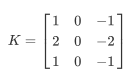
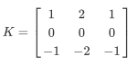
The Sobel filter can extract edges in a specific direction (vertical or horizontal). For the sobel filter, please refer to OpenCV: Image Filtering. The filter is defined as follows:
Portrait:

Horizontal:
img = cv2.cvtColor(img, cv2.COLOR_BGR2GRAY)
img_x = cv2.Sobel(img, cv2.CV_64F, 1, 0)
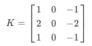
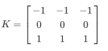
img_y = cv2.Sobel(img, cv2.CV_64F, 0, 1)16. Prewitt filter
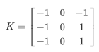
Prewitt filter is a filter used for edge detection. Its function can be referred tohttps://docs.scipy.org/doc/scipy/reference/generated/ scipy.ndimage.prewitt.html
Portrait:
Horizontal:
img = cv2.cvtColor(img, cv2.COLOR_BGR2GRAY)
img_x = scipy.ndimage.prewitt(img, 1)
img_y = scipy.ndimage.prewitt(img, 0)
17. Laplacian filter
The Laplacian filter is a filter that differentiates the image brightness twice to detect edges. https://docs.opencv.org/master/d4/d86/group__imgproc__filter.html#gad78703e4c8fe703d479c1860d76429e6
Portrait:
Horizontal:
img = cv2.cvtColor(img, cv2.COLOR_BGR2GRAY)
img = cv2.Laplacian(img,cv2.CV_64F)
18. Emboss filter
Emboss filter can make object outlines clearer
img = cv2.cvtColor(img, cv2.COLOR_BGR2GRAY)
kernel = np.array([[-2, -1, 0], [-1, 1, 1], [0, 1, 2]])
img = cv2.filter2D(img, -1, kernel)
19. Log filter
LoG is the abbreviation of Laplacian of Gaussian. The Gaussian filter is used to smooth the image and then the Laplacian filter is used to make the outline of the image clearer. Its functions can be referred tohttps://docs.scipy.org/doc/scipy/reference/generated/scipy.ndimage.gaussian_laplace.html
img = cv2.cvtColor(img, cv2.COLOR_BGR2GRAY)
img = scipy.ndimage.gaussian_laplace(img, sigma=3)
20. Histogram drawing
Draw a histogram showing the number of occurrences of pixels with different values. The hist() function in Matplotlib provides an interface for drawing histograms. https://matplotlib.org/api/_as_gen/matplotlib.pyplot.hist.html
img = cv2.imread('imori_dark.jpg').astype(np.float)
plt.hist(img.ravel(), bins=255, rwidth=0.8, range=(0, 255))
plt.savefig("answer.png")
21. Histogram equalization
Histogram equalization is a method of enhancing image contrast. Its main idea is to change the histogram distribution of an image into an approximately uniform distribution. Its referencehttps://stackoverflow.com/questions/31998428/opencv-python-equalizehist-colored-image
img_yuv = cv2.cvtColor(img, cv2.COLOR_BGR2YUV)
# equalize the histogram of the Y channel
img_yuv[:,:,0] = cv2.equalizeHist(img_yuv[:,:,0])
# convert the YUV image back to RGB format
img_output = cv2.cvtColor(img_yuv, cv2.COLOR_YUV2BGR)
22. Gamma correction
Gamma correction is used to correct the nonlinear conversion characteristics of sensors in electronic devices such as cameras. If the image is displayed on the monitor, the picture will appear very dark. Gamma correction eliminates the influence of the display by pre-increasing the RGB value to achieve the purpose of image correction. Its referencehttps://stackoverflow.com/questions/33322488/how-to-change-image-illumination-in-opencv-python/41061351
def adjust_gamma(image, gamma=1.0):

   invGamma = 1.0 / gamma
   table = np.array([((i / 255.0) ** invGamma) * 255
      for i in np.arange(0, 256)]).astype("uint8")

   return cv2.LUT(image, table)

original = cv2.imread('imori_gamma.jpg')
gamma = 2.2
adjusted = adjust_gamma(original, gamma=gamma)
cv2.imwrite('answer.png', adjusted)
23. Common interpolation methods
Includes bicubic, bilinear, and nearest neighbor interpolation.
img = cv2.imread('imori.jpg')
height, width = img.shape[:2]
new_height, new_width = int(height/2), int(width/2)
# 双三次
new_img = cv2.resize(img, (new_width, new_height), interpolation=cv2.INTER_CUBIC)
# 双线性
new_img = cv2.resize(img, (new_width, new_height), interpolation=cv2.INTER_LINEAR)
# 最邻近
new_img = cv2.resize(img, (new_width, new_height), interpolation=cv2.INTER_NEAREST)