0. Summary
We propose a new method for efficient and high-quality object and scene image segmentation. By analogizing classical computer graphics methods to the oversampling and undersampling challenges faced in pixel labeling tasks, we develop a unique perspective on image segmentation as a rendering problem. Based on this perspective, we propose the PointRend (Point-based Rendering) neural network module: a module that performs point-based segmentation predictions at adaptively selected locations based on an iterative subdivision algorithm. PointRend can be flexibly applied to instance segmentation and semantic segmentation tasks by building on top of existing state-of-the-art models. While many specific implementations are possible, we show that a simple design can already achieve excellent results. Qualitatively, PointRend outputs clear object boundaries in areas where previous methods were over-smoothed. Quantitatively, PointRend brings significant gains for instance segmentation and semantic segmentation on COCO and Cityscapes. PointRend's efficiency makes the output resolution more practical in terms of memory or computation than existing methods. The code has been made available at https://github.com/facebookresearch/detectron2/tree/master/projects/PointRend.
1 Introduction
The image segmentation task involves mapping pixels sampled on a regular grid to a label map or set of label maps on the same grid. In the case of semantic segmentation, the label map indicates the predicted class of each pixel. In the case of instance segmentation, a binary foreground versus background map is predicted for each detected object. Modern tools for these tasks are built on convolutional neural networks (CNN) [24, 23]. CNNs for image segmentation typically operate on regular grids: the input images are regular grids of pixels, their hidden representations are feature vectors on the regular grid, and their outputs are label maps on the regular grid. Regular grids are convenient but not necessarily computationally ideal for image segmentation. The label maps predicted by these networks should be mostly smooth, i.e. adjacent pixels usually take the same label, because high-frequency regions are restricted to sparse boundaries between objects. A regular grid will unnecessarily oversample smooth areas while undersampling object boundaries. The result is overcomputed and blurred contours in smooth areas (Figure 1, top left). Image segmentation methods typically predict labels on a low-resolution regular grid, e.g., 1/8 of the input in semantic segmentation [30] or 28 × 28 in instance segmentation [17], to achieve a balance between undersampling and oversampling. make a compromise.
Similar sampling problems have been studied in computer graphics for decades. For example, the renderer maps a model (for example, a three-dimensional mesh) to a rasterized image, a regular grid of pixels. Although the output is on a regular grid, the calculations are not evenly distributed on the grid. Instead, a common graphics strategy is to compute pixel values for an irregular subset of adaptively selected points on the image plane. For example, the classic subdivision technique of [43] produces a quadtree-like sampling pattern that can efficiently render high-resolution anti-aliased images. The core idea of this paper is to treat image segmentation as a rendering problem and borrow classic ideas from computer graphics to efficiently "render" high-quality label maps (see Figure 1, lower left corner). We encapsulate this computational idea in a new neural network module called PointRend, which uses a segmentation strategy to adaptively select non-uniform point sets for computing labels. PointRend can be integrated into popular meta-architectures for instance segmentation (e.g., Mask R-CNN [17]) and semantic segmentation (e.g., FCN [30]). Its segmentation strategy uses an order of magnitude fewer floating-point operations than direct intensive computation to efficiently compute high-resolution segmentation maps.
PointRend is a general module with many possible implementations. Viewed abstractly, a PointRend module accepts one or more typical CNN feature maps f(xi,yi) defined on a regular grid and outputs high-resolution predictions p(x′i, yi′). PointRend does not overpredict all points on the output grid, but only predicts on carefully selected points. To make these predictions, it extracts point-wise feature representations of selected points by interpolating f and uses a small nod sub-network to predict output labels from the point-wise features. We will provide a simple yet efficient implementation of PointRend. We use the COCO [26] and Cityscapes [8] benchmarks to evaluate the performance of PointRend in instance segmentation and semantic segmentation tasks. In terms of quality, PointRend is able to efficiently calculate sharp boundaries between objects, as shown in Figures 2 and 8. We also observe quantitative improvements, although the standard intersection-over-union ratio metrics for these tasks (mask AP and mIoU) are biased towards intra-object pixels and are relatively insensitive to boundary improvements. PointRend significantly improves the powerful Mask R CNN and DeepLabV3 [4] models.
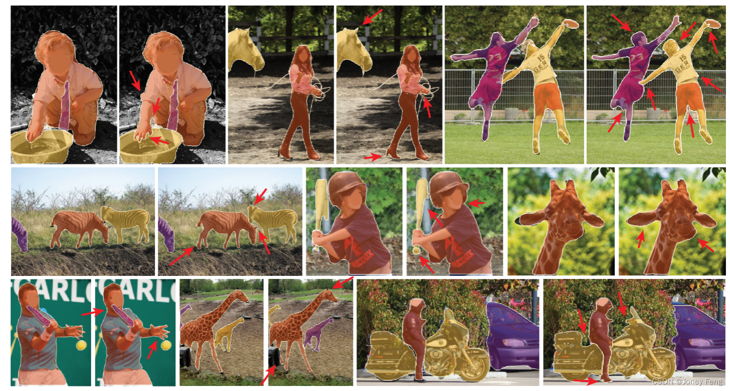
Figure 2: Example results using ResNet-50 [18] and FPN [25] using Mask R-CNN [17] with a standard mask head (left) versus using PointRend (right). Note that PointRend predicts masks with finer detail around object boundaries.
2.Related work
Rendering algorithms in computer graphics output a regular grid of pixels. However, they usually compute these pixel values on non-uniform point sets. Efficient procedures like subdivision [43] and adaptive sampling [33, 37] can refine coarse rasterizations in areas with large variance in pixel values. Ray tracing renderers often use supersampling [45], a technique that samples certain points more densely than the output mesh to avoid aliasing effects. Here we apply classic subdivision to image segmentation. Non-uniform grid representation. In 2D image analysis, regular grid-based computation is the dominant paradigm, but this is not the case for other vision tasks. In 3D shape recognition, large 3D grids are not feasible due to cube scaling. Most CNN-based methods do not exceed a coarse grid of 64×64×64 [11,7]. In contrast, recent works consider more efficient non-uniform representations such as grids [42, 13], signed distance functions [32] and oc-trees [41]. Similar to the signed distance function, PointRend can calculate split values at any point. Recently, Marin et al. [31] proposed an efficient semantic segmentation network based on non-uniform subsampling of the input image, which is then processed using a standard semantic segmentation network. In contrast, PointRend focuses on non-uniform sampling at output. It may be possible to combine these two methods, but [31] has not yet been proven suitable for instance segmentation.
Instance segmentation methods based on the Mask R-CNN meta-architecture [17] have occupied the top positions in recent challenges [29, 2]. These region-based architectures typically predict masks on a 28×28 grid, regardless of object size. This is sufficient for small objects, but for large objects it produces undesirable "blobby" output, over-smoothing the details of large objects (see Figure 1, top left). On the other hand, bottom-up methods group pixels into object masks [28, 1, 22]. These methods can produce more detailed output but lag behind region-based methods on most instance segmentation benchmarks [26, 8, 35]. TensorMask [6] is an alternative sliding window method that uses a complex network design to predict clear high-resolution masks for large objects, but it is also slightly less accurate. In this paper, we show that a region-based segmentation model equipped with PointRend can produce masks with a level of detail while improving the accuracy of region-based methods.
Semantic segmentation. Fully Convolutional Networks (FCNs) [30] are the basis of modern semantic segmentation methods. They typically predict the output to be at a lower resolution than the input grid and use bilinear upsampling to recover the remaining 8-16× resolution. Results can be improved by replacing dilated/atrous convolutions [3, 4] with some downsampling layers, but at the cost of more memory and computation. Alternative approaches include encoder-decoder architectures [5, 21, 39, 40], where the encoder downsamples the grid representation and then upsamples it in the decoder, using skip connections [39] to recover filtered details . Current methods combine dilated convolutions with an encoder-decoder structure [5, 27], producing the output on a grid 4× sparser than the input grid before applying bilinear interpolation. In our work, we propose a method to efficiently predict the level of detail on meshes that are as dense as the input mesh.
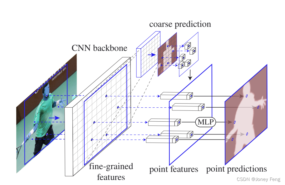
Figure 3: PointRend applied to instance segmentation. The standard instance segmentation network (solid red arrow) accepts an input image and uses a lightweight segmentation head to produce a coarse (e.g. 7×7) mask prediction for each detected object (red box). To refine the coarse mask, PointRend selects a set of points (red points) and uses a small MLP to predict each point independently. The MLP uses interpolated features of these points calculated from (1) the fine-grained feature map of the backbone CNN and (2) the coarse prediction mask (dashed red arrow). Coarse mask features enable MLP to make different predictions on a single point containing two or more boxes. The proposed subdivision mask rendering algorithm (see Figure 4 and §3.1) applies this process iteratively to refine the uncertain regions of the predicted mask.
3.Method
We analogize image segmentation (objects and/or scenes) in computer vision to image rendering in computer graphics. Rendering is about displaying a model (for example, a 3D mesh) as a regular mesh of pixels, i.e. an image. While the output representation is a regular mesh, the underlying physical entity (e.g., 3D model) is continuous and its physical occupancy and other properties can be mapped to any real-valued point on the image plane using physical and geometric reasoning (such as ray tracing) Make an inquiry. By analogy, in computer vision, we can think of image segmentation as an occupancy map of the underlying continuous entities, and from this "render" the segmentation output, which is a regular grid of predicted labels. This entity is encoded in the feature map of the network and can be accessed at any point through interpolation. A parameterized function that is trained to predict occupancy through these interpolated point feature representations is the counterpart of physical and geometric reasoning.
Based on this analogy, we propose PointRend (point-based rendering) as an image segmentation method using point representation. A PointRend module accepts one or more C-channel typical CNN feature maps f ∈ RC×H×W, each feature map is defined on a regular grid (usually 4 to 16 times coarser than the image grid), and outputs Prediction of K class labels p∈RK×H′×W′ on a regular grid at different (possibly higher) resolution. The PointRend module consists of three main components: (i) Point selection strategy selects a small number of real-valued points for prediction, avoiding overcomputation of all pixels in the high-resolution output grid. (ii) For each selected point, extract point feature representation. Characteristics of real-valued points are calculated by bilinear interpolation of f, using the 4 nearest neighbors of the point on the normal grid of f. Therefore, it is able to exploit the sub-pixel information encoded in the channel dimensions of f to predict segmentations with higher resolution than f. (iii) Nod: a small neural network trained to predict the label of each point. The PointRend architecture can be applied to instance segmentation (e.g., Mask R-CNN [17]) and semantic segmentation (e.g., FCN [30]) tasks. For instance splitting, PointRend is applied to each region. It computes the mask in a coarse-to-fine manner by making predictions on a selected set of points (see Figure 3). For semantic segmentation, the entire image can be considered as a single region, so without loss of generality, we will describe PointRend in the context of instance segmentation. Next, we discuss the three main components in detail.
3.1. Point selection for inference and training
The core idea of our method is to flexibly and adaptively select points on the image plane that predict segmentation labels. Intuitively, these points should be located more densely near high-frequency regions, such as object boundaries, similar to the anti-aliasing problem in ray tracing. We developed this idea for both inference and training. infer. Our inference selection strategy is inspired by adaptive subdivision in computer graphics [43]. This technique is used to compute a high-resolution image (for example, by ray tracing) only at locations where the possible values differ significantly from their neighbors, for all other locations the values are obtained by interpolating the already computed output values (from a coarse grid start).
For each region, we iteratively "render" the output mask in a coarse-to-fine fashion. The coarsest level predictions are made at points on a regular grid (e.g., by using a standard coarse segmentation prediction head). At each iteration, PointRend upsamples its previously predicted segmentations using bilinear interpolation and then selects the N most uncertain points on this denser grid (e.g., for a binary mask, the one with probability closest to 0.5 point). PointRend then computes point feature representations for each of these N points (described later in §3.2) and predicts their labels. This process is repeated until the segmentation is upsampled to the desired resolution. One step of this process is illustrated in the toy example of Figure 4. For a required output resolution of M × M pixels and a starting resolution of M0 × M0, PointRend requires no more point predictions than N log2 MM0. This is much smaller than M×M, enabling PointRend to make high-resolution predictions more efficiently. For example, if M0 is 7 and the required resolution is M=224, 5 subdivision steps are required. If we choose N = 282 points at each step, PointRend only makes predictions for 282 4.25 points, which is 15 times smaller than 2242. Note that the overall number of points selected is less than N log2 MM0 because in the first subdivision step, only 142 points are available.
During training, PointRend also needs to select points to build point features for training nodding. In principle, point selection strategies can be similar to the segmentation strategies used in inference. However, segmentation introduces sequential steps that are not conducive to training neural networks using backpropagation. Instead, during training, we use a non-iterative strategy based on random sampling. The sampling strategy selects N points on the feature map for training. It aims to bias selection in areas of uncertainty while maintaining a degree of uniform coverage, using three principles. (i) Overgeneration: We overgenerate candidate points by randomly sampling kN points (k>1) from a uniform distribution. (ii) Importance sampling: We focus on points with uncertain coarse predictions by interpolating the coarse prediction values across all kN points and computing task-specific uncertainty estimates (defined in §4 and §5). Select the most uncertain βN points (β∈[0,1]) from kN candidate points. (iii) Coverage: The remaining (1−β)N points are sampled from a uniform distribution. We illustrate this process in Figure 5 using different settings and compare it with regular mesh selection. At training time, the prediction and loss functions are calculated only on N sample points (except for coarse segmentation), which is simpler and more efficient than backpropagation through the segmentation step. This design is similar to the parallel training of RPN + Fast R-CNN in the Faster R-CNN system [12], and its inference is sequential.
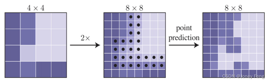
Figure 4: An example of an adaptive segmentation step. Predictions on a 4×4 grid are upsampled by 2× using bilinear interpolation. PointRend then makes predictions on the N most blurry points (black points) to recover details on a finer grid. This process is repeated until the desired grid resolution is achieved.
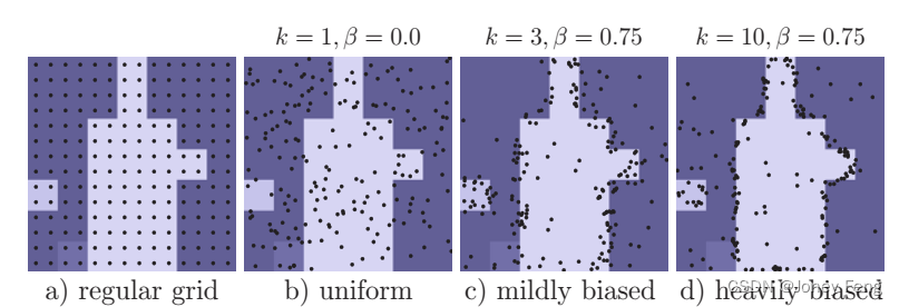 Figure 5: Point sampling during training. We show N = 142 points sampled using different strategies, corresponding to the same underlying rough prediction. In order to achieve high performance, only a small number of points are sampled in each area, and a slightly biased sampling strategy is adopted to make the system more efficient during the training process.
3.2. Pointing and nodding
PointRend constructs point features on selected points by combining (e.g., concatenating) two feature types, namely fine-grained and coarse prediction features, described below. Fine-grained features: To allow PointRend to render fine segmentation details, we extract a feature vector at each sampling point from the CNN feature map. Because a point is a real-valued 2D coordinate, we perform bilinear interpolation on the feature map to compute the feature vector, following standard practice [19, 17, 9]. Features can be extracted from a single feature map (e.g. res2 in ResNet); they can also be extracted and concatenated from multiple feature maps (e.g. res2 to res5 or their feature pyramid [25] counterparts), following the Hypercolumn approach [15 ]. Coarse Predictive Features: Fine-grained features make it feasible to resolve details, but have drawbacks in two aspects. First, they do not contain region-specific information, so the same point where the bounding boxes of two instances overlap will have the same fine-grained features. However, the point can only be in the foreground of one instance. Therefore, for instance segmentation tasks, different regions may predict different labels for the same point, requiring additional region-specific information.
Second, depending on the feature map used for fine-grained features, the features may only contain relatively low-level information (for example, we will use res2 from DeepLabV3). In this case, a feature source with more contextual and semantic information may be helpful. This issue affects both instance and semantic segmentation. Based on these considerations, the second feature type is the coarse segmentation prediction from the network, i.e., a K-dimensional vector representing each point in each region (box) predicted by K classes. By design, coarse resolution provides a more global context, while channels convey semantic categories. These rough predictions are similar to the output produced by existing architectures and are supervised during training in the same way as existing models. For instance segmentation, the coarse prediction can be e.g. the output of a lightweight 7×7 resolution mask head in Mask R-CNN. For semantic segmentation, it can be e.g. predictions from stride 16 feature maps. nod. Given the point-level feature representation of each selected point, PointRend uses a simple multi-layer perceptron (MLP) for point-level segmentation prediction. This MLP shares weights among all points (and all regions), similar to graph convolution [20] or PointNet [38]. Since MLP predicts segmentation labels for each point, it can be trained with standard task-specific segmentation losses (described in §4 and §5).
4. Experiment: Instance Segmentation
data set. We use two standard instance segmentation datasets: COCO [26] and Cityscapes [8]. We report the standard masked AP metric [26] for 3 runs of COCO and 5 runs of Cityscapes using the median (which has higher variance). COCO has 80 categories with instance-level annotations. We train on train2017 (~118k images) and report results on val2017 (5k images). As stated in [14], the ground truth of COCO is often rough and the AP of the dataset may not fully reflect the improvement in mask quality. Therefore, we use the 80 COCO category subset of LVIS [14] for AP supplementation, denoted as AP!. The annotation quality of LVIS is significantly higher. Note that for AP!, we use the same model trained on COCO and re-evaluate its predictions using the LVIS evaluation API to evaluate against higher quality LVIS annotations. Cityscapes is an egocentric street view dataset with 8 categories, 2975 training images and 500 validation images. Compared to COCO, these images have higher resolution (1024 × 2048 pixels) and have finer and more pixel-accurate ground instance segmentation annotations.
Architecture. Our experiments demonstrate Mask R-CNN using the ResNet-50 [18] + FPN [25] backbone network. The default mask head in Mask R-CNN is region-level FCN, which we denote as “4×conv”. 2We use this as a baseline for comparison. For PointRend, we make appropriate modifications to this baseline, which are described below. A lightweight, coarse mask prediction header. To compute coarse predictions, we replace the 4×conv mask header with a more lightweight design, similar to that of Mask R-CNN, and produce a 7×7 mask prediction. Specifically, for each bounding box, we extract a 14 × 14 feature map from the P2 level of FPN using bilinear interpolation. Features are computed on a regular grid within the bounding box (this operation can be seen as a simple version of RoIAlign). Next, we use a 2×2 convolutional layer with stride 2, with 256 output channels, followed by ReLU [34], reducing the spatial size to 7×7. Finally, similar to the Mask R-CNN box header, an MLP with two 1024-wide hidden layers is applied to produce 7 × 7 mask predictions for each K class. Use ReLU in the hidden layer of the MLP and apply a sigmoid activation function to its output. PointRend. At each selection point, a K-dimensional feature vector is extracted from the output of the coarse prediction head using bilinear interpolation. PointRend also uses bilinear interpolation to extract a 256-dimensional feature vector from the P2 level of FPN. This level has 4 steps relative to the input image. These coarse predictions and fine-grained feature vectors are concatenated. We use MLP with 3 hidden layers with 256 channels for K-class prediction at selected points. In each layer of the MLP, we supplement the 256 output channels with K coarse prediction features to make the input vectors used for the next layer. We use ReLU inside the MLP and apply sigmoid to its output.
train. We default to using the standard 1× training plan and data augmentation of Detectron2 [44] (full details in the Appendix). For PointRend, we randomly sample 142 points using a biased sampling strategy of k = 3 and β = 0.75. We use the distance between the interpolated from the coarse prediction and 0.5 of the ground instance segmentation class probability as the point-level uncertainty measure. For a predicted box with ground instance segmentation class c, we sum the binary cross-entropy loss of the c-th MLP output over 142 points. The lightweight coarse prediction head predicts the mask for class c using an average cross-entropy loss, i.e. the same loss as the baseline 4×conv head. We sum all losses without any reweighting. During training, Mask R-CNN applies boxes and masks in parallel, while during inference they run as a cascade. We find that cascade training does not improve the baseline Mask R-CNN, but PointRend can benefit from it because it samples points within more accurate boxes, slightly improving overall performance (~0.2% AP, absolute). reasoning. For predicted boxes of category c, without special instructions, we use adaptive segmentation technology to optimize the rough 7×7 prediction of category c to 224×224, which takes 5 steps. At each step, we select and update (at most) N = 282 most uncertain points based on the absolute difference between the predicted value and 0.5.
4.1. Main results
We compare PointRend with the default 4×conv head in Mask R-CNN in Table 1. PointRend outperforms the default header on both datasets. When evaluating the COCO class using LVIS annotations (AP!), as well as on Cityscapes, the gap is larger, which we attribute to the superior annotation quality in these datasets. Even with the same output resolution, PointRend outperforms the baseline. The difference between 28×28 and 224×224 is relatively small because AP uses the intersection-and-union ratio [10] and is therefore heavily biased towards internal object pixels and less sensitive to boundary quality. Visually, however, the difference in boundary quality is evident, see Figure 6.
Subdivision inference allows PointRend to use 30x more computation (FLOPs) and memory to produce high-resolution 224×224 predictions, while the default 4×conv header needs to output the same resolution (based on taking a 112×112 RoIAlign input), see Table 2 . PointRend makes high-resolution output a feasible solution in the Mask R-CNN framework by ignoring regions where the coarse prediction of the object is sufficient (e.g., regions far away from the object boundary). In terms of wall clock runtime, our unoptimized implementation outputs a 224×224 mask at ∼13 fps, which is about the same as a 4×conv header modified to output a 56×56 mask (by doubling the default RoIAlign size) The frame rate, in fact, this design has lower COCO AP compared to the 28×28 4×conv head (34.5% vs. 35.2%). Table 3 shows PointRend segmentation inference for selecting different output resolutions and number of points in each segmentation step. Predicting masks at higher resolutions improves results. Despite AP saturation, visual improvements are still evident when outputting from lower (e.g., 56×56) to higher (e.g., 224×224) resolutions, see Figure 7. Since points are selected first in the fuzzy areas, the AP will also saturate as the number of points sampled in each subdivision step increases. Additional points may be predicted in areas where the prediction is already coarse enough. However, for objects with complex boundaries, using more points may be beneficial.
Table 1: Comparison of PointRend with the default 4× convolution mask header of Mask R-CNN [17]. Mask AP reported. AP! is an evaluation of COCO mask AP on higher quality LVIS annotations [14] (see text for details). Both COCO and Cityscapes models use the ResNet-50-FPN backbone network. PointRend outperforms standard 4× convolution mask points both quantitatively and qualitatively, with higher output resolution leading to more detailed predictions, see Figures 2 and 6.

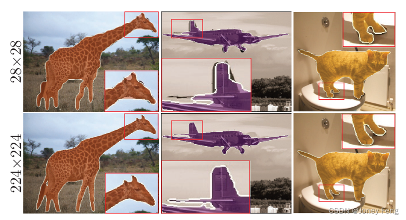
Figure 6: PointRend inference using different output resolutions. High-resolution masks align better with object boundaries.
Table 2: FLOPs (multiplication-add) and activation counts for 224×224 output resolution mask. PointRend's efficient subdivision makes 224×224 output possible, while the standard 4× convolution mask bit is modified to use a RoIAlign size of 112×112.
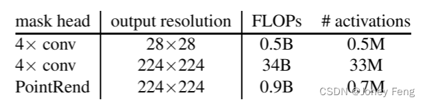
Table 3: Segmentation inference parameters. Higher output resolution improves AP. Although the number of points sampled per subdivision step saturates quickly at underline values, the quality results may continue to improve for complex objects. AP! is an evaluation of COCO mask AP on higher quality LVIS annotations [14] (see text for details). 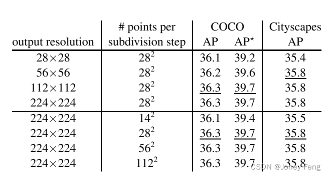
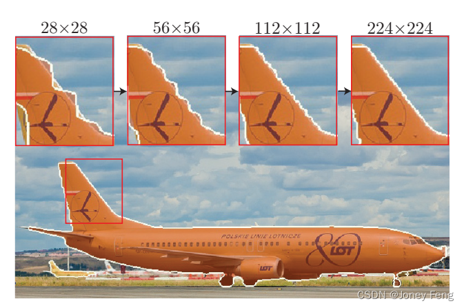 Figure 7: PointRend’s anti-aliasing. Accurate object hooking delin requires the output mask resolution to match or exceed the resolution of the input image area occupied by the object.
Table 4: Training time point selection strategy using 142 points per box. Sampling that is slightly biased toward the uncertain region works best. Heavily biased sampling performs even worse than uniform or regular grid sampling, indicating the importance of coverage. AP! is an evaluation of COCO mask AP on higher quality LVIS annotations [14] (see text for details).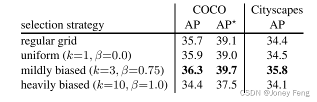
Table 5: Larger model and longer 3× schedule [16]. PointRend benefits from more advanced models and longer training times. The gap between PointRend and the default masked points in Mask R-CNN remains unchanged. AP! is an evaluation of COCO mask AP on higher quality LVIS annotations [14] (see text for details).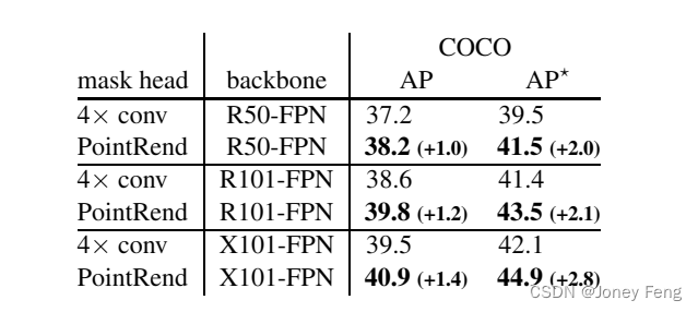
4.2.Ablation experiment
We conducted a number of analyzes to analyze PointRend. Overall, we note that it is robust to the exact design of the nod MLP. In our experiments, changes in its depth or width did not show any significant difference. Point selection during training. During training, we select 142 points per object following a biased sampling strategy (§3.1). Sampling only 142 points makes training computationally and memory efficient, we found that using more points does not improve the results. Surprisingly, sampling only 49 points per box still maintains AP, although we observe increased variance in AP. Table 4 shows the performance of PointRend under different selection strategies. During training, regular grid selection achieves results similar to uniform sampling. And biased sampling towards blurred areas can improve AP. However, a sampling strategy that favors roughly predicted boundaries too much (k > 10 and β close to 1.0) will reduce AP. Overall, we find that a wide range of parameters 2<k<5 and 0.75<β<1.0 provide similar results. Bigger model, longer training. Training ResNet-50+FPN (denoted as R50-FPN) on COCO using 1× scheduling leads to underfitting. In Table 5, we show that PointRend’s improvements over the baseline persist on longer training schedules and larger models (see Appendix for details).
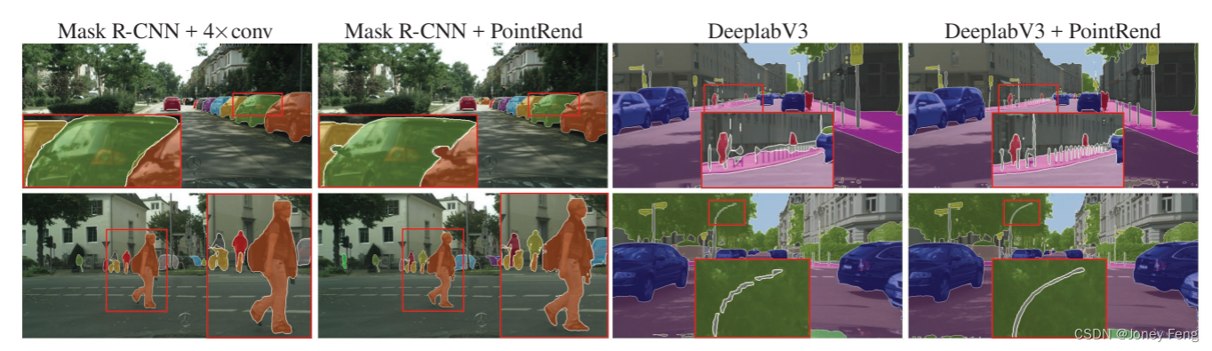 Figure 8: Cityscapes example results for instance segmentation and semantic segmentation. In instance segmentation, larger objects benefit more from PointRend producing high-resolution output. For semantic segmentation, PointRend can recover small objects and details.
5. Experiment: Semantic Segmentation
PointRend is not limited to instance segmentation, but can also be extended to other pixel-level recognition tasks. Here, we show how PointRend benefits from two semantic segmentation models: DeeplabV3 [4] which uses dilated convolutions to predict on a denser grid, and SemanticFPN [21], a simple encoder-decoder structure. data set. We use the Cityscapes [8] semantic segmentation set containing 19 categories, 2975 training images, and 500 validation images. We report the median mIoU over 5 trials. Implementation details. We reimplemented DeeplabV3 and SemanticFPN, following their respective papers. SemanticFPN uses standard ResNet-101 [18], while DeeplabV3 uses ResNet-103 proposed in [4]. We follow the training plan and data augmentation of the original paper (see Appendix for details). We use the same PointRend architecture as instance splitting. Coarse predicted features come from the (already coarse) output of a semantic segmentation model. Fine-grained features are interpolated from res2 to DeeplabV3 and from P2 interpolation to SemanticFPN. During training, we sample the same number of points as those on the input stride 16 feature map (2304 for deeplabV3 and 2048 for SemanticFPN). We use the same k=3, β=0.75 point selection strategy. During inference, tessellation uses N=8096 (i.e. the number of points in the stride 16 map of a 1024×2048 image) until the input image resolution is reached. To measure prediction uncertainty, we use the same strategy during training and inference: the difference between the most and least confident class probabilities.
In DeeplabV3, Table 6 compares DeepLabV3 and DeeplabV3 with PointRend. The output resolution can also be increased by a factor of 2 by using dilated convolutions in the res4 stage, described in [4]. Compared with the two, PointRend has higher mIoU. Qualitative improvements are also evident, see Figure 8. By adaptively sampling points, PointRend can achieve 1024×2048 resolution (i.e. 2M points) by making predictions on only 32k points, see Figure 9. SemanticFPN. Table 7 shows that SemanticFPN with PointRend improves over both the 8× and 4× output stride variants without PointRend.
Table 6: Cityscapes semantic segmentation using PointRend’s DeepLabV3 outperforms baseline DeepLabV3. Scaling up the res4 stage during inference yields larger, more accurate predictions, but at a much higher computational and storage cost; still not as good as using PointRend.

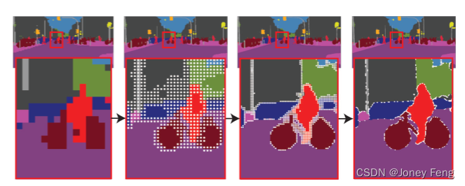
Figure 9: PointRend inference for semantic segmentation. PointRend refines prediction scores for areas where coarse predictions are insufficient. To visualize the score at each step, we take arg max at a given resolution without bilinear interpolation.
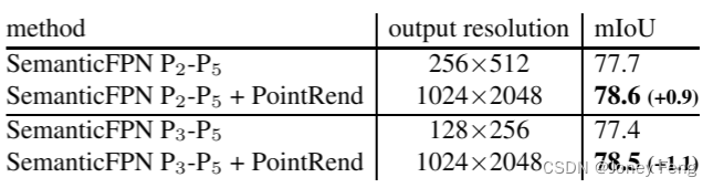
Table 7: Cityscapes semantic segmentation using PointRend’s SemanticFPN outperforms baseline SemanticFPN.