NumPy is one of the core packages for numerical calculations in Python. It provides a large number of efficient array operation functions and mathematical functions. It supports multi-dimensional array and matrix operations, and can integrate C/C++ and Fortran codes, so it can process large amounts of data very efficiently. Here are some of the main features and uses of NumPy:
-
Multidimensional array: The core of NumPy is the ndarray (N-dimensional array) object, which can be used to store elements of the same type. These arrays can be one, two or higher dimensional. They provide convenient array indexing and slicing, as well as many basic operations and calculations (such as addition, subtraction, multiplication, division, exponentiation, etc.).
-
Array operations: NumPy provides a large number of array operation functions, including mathematical functions (such as trigonometric functions, exponential functions, logarithmic functions, etc.), logical functions (such as Boolean operations, comparison operations, logical operations, etc.), sorting functions, statistical functions, etc. .
-
Matrix operations: NumPy provides matrix operation functions, such as matrix addition, subtraction, multiplication, transpose, inversion, etc., which can easily perform linear algebra calculations.
-
Random number generation: NumPy can generate various random numbers, such as normal distribution, uniform distribution, Poisson distribution, Bernoulli distribution, etc., as well as random permutation and random selection.
-
File IO: NumPy can read and write various file formats, including text files, binary files, and matlab files, to facilitate data storage and transmission.
-
Integration with other Python libraries: NumPy can be easily integrated with other Python libraries (such as Pandas, SciPy, matplotlib, etc.) for data analysis, scientific computing, and visualization.
import numpy as npNdarray
1. Operation of ndarray
Generate list data into array()
a = np.array([1,2,3,4,5])Confirm data type
print(a.dtype) # int32If you substitute a floating point number into an integer array, the data will automatically become an integer (the decimal point will be automatically rounded off)
a[1] = -3.6
print(a)  # [1 -3 3 4 5]
Transform data type
a2 = a.astype(np.float32)
print(a2, a2.dtype)  # [1. -3. 3. 4. 5.] float32
Two-dimensional array
b = np.array([[1, 2, 3],
              [3.2, 5.3, 6.6]])
print('b=', b)  # b= [[1.  2.  3. ][3.2 5.3 6.6]]
print('b[1,2]=', b[1,2])  # b[1,2] = 6.6
2.ndarray parameters
- ndarry.ndim The dimensionality of the array
- ndarry.shape Number of rows and columns of the array
- ndarry.size The number of elements
- ndarry.dtype Data type
print('ndim =', a.ndim, b.ndim)
print('shape =', a.shape, b.shape)
print('size =', a.size, b.size)
print('dtype =', a.dtype, b.dtype)

# ndim = 1 2
# shape = (5,) (2, 3)
# size = 5 6
# dtype = float32 float64
reshape reorganizes the array (the number of elements remains unchanged)
print(b.reshape(6)) # 转为1维数组 [ 1.   2.  -1.1  3.2  5.3  6.6]
print(b.reshape(3,2)) # 转为3行2列数组 [[ 1.   2. ][-1.1  3.2][ 5.3  6.6]]
print(b.T) # 矩阵的转置 [[ 1.   3.2][ 2.   5.3][-1.1  6.6]]
Matrix calculations
When performing four arithmetic operations on matrices and numerical values, operations are performed on each value.
print(b+2)  #[[3.  4.  0.9][5.2 7.3 8.6]]
print(b-2)  #[[-1.   0.  -3.1][ 1.2  3.3  4.6]]
print(b*2)  #[[ 2.   4.  -2.2][ 6.4 10.6 13.2]]
print(b/2)  #[[ 0.5   1.   -0.55][ 1.6   2.65  3.3 ]]
print(b**3) #3次幂 [[  1.      8.     -1.331][ 32.768 148.877 287.496]]
print(b//1) #用这种方法舍掉小数 [[ 1.  2. -2.][ 3.  5.  6.]]
When calculating matrices of the same dimension, the values at the same position are calculated (an error will be reported if the matrix dimensions are different)
c = b/2
print(b+c)  # [[ 1.5   3.   -1.65][ 4.8   7.95  9.9 ]]
print(b-c)  # [[ 0.5   1.   -0.55][ 1.6   2.65  3.3 ]]
print(b*c)  # [[ 0.5    2.     0.605][ 5.12  14.045 21.78 ]]
print(b/c)  # [[2. 2. 2.][2. 2. 2.]]
The product of matrices is "@"
a-row, b-row x b-row, c = a-row, c-column matrix
A = np.arange(6).reshape(3,2)
B = np.arange(8).reshape(2,4)
print(A)  #[[0 1][2 3][4 5]]
print(B)  #[[0 1 2 3][4 5 6 7]]
print(A@B)  #[[ 4  5  6  7][12 17 22 27][20 29 38 47]]
Generation of matrix
Generation of 1-dimensional matrix (initial value, end value, conditions)
- The arange condition is the specified step size, and the total number is automatically determined, excluding the end value.
- The linspace condition is the total number, and the step size is automatically determined, including the end value.
np.arange(0,10,0.1)
# array([0. , 0.1, 0.2, 0.3, 0.4, 0.5, 0.6, 0.7, 0.8, 0.9, 1. , 1.1, 1.2,
#      1.3, 1.4, 1.5, 1.6, 1.7, 1.8, 1.9, 2. , 2.1, 2.2, 2.3, 2.4, 2.5,
#      2.6, 2.7, 2.8, 2.9, 3. , 3.1, 3.2, 3.3, 3.4, 3.5, 3.6, 3.7, 3.8,
#      3.9, 4. , 4.1, 4.2, 4.3, 4.4, 4.5, 4.6, 4.7, 4.8, 4.9, 5. , 5.1,
#      5.2, 5.3, 5.4, 5.5, 5.6, 5.7, 5.8, 5.9, 6. , 6.1, 6.2, 6.3, 6.4,
#      6.5, 6.6, 6.7, 6.8, 6.9, 7. , 7.1, 7.2, 7.3, 7.4, 7.5, 7.6, 7.7,
#      7.8, 7.9, 8. , 8.1, 8.2, 8.3, 8.4, 8.5, 8.6, 8.7, 8.8, 8.9, 9. ,
#      9.1, 9.2, 9.3, 9.4, 9.5, 9.6, 9.7, 9.8, 9.9])

np.linspace(0,10,100)
# array([ 0. ,  0.1,  0.2,  0.3,  0.4,  0.5,  0.6,  0.7,  0.8,  0.9,  1. ,
#       1.1,  1.2,  1.3,  1.4,  1.5,  1.6,  1.7,  1.8,  1.9,  2. ,  2.1,
#       2.2,  2.3,  2.4,  2.5,  2.6,  2.7,  2.8,  2.9,  3. ,  3.1,  3.2,
#       3.3,  3.4,  3.5,  3.6,  3.7,  3.8,  3.9,  4. ,  4.1,  4.2,  4.3,
#       4.4,  4.5,  4.6,  4.7,  4.8,  4.9,  5. ,  5.1,  5.2,  5.3,  5.4,
#       5.5,  5.6,  5.7,  5.8,  5.9,  6. ,  6.1,  6.2,  6.3,  6.4,  6.5,
#       6.6,  6.7,  6.8,  6.9,  7. ,  7.1,  7.2,  7.3,  7.4,  7.5,  7.6,
#       7.7,  7.8,  7.9,  8. ,  8.1,  8.2,  8.3,  8.4,  8.5,  8.6,  8.7,
#       8.8,  8.9,  9. ,  9.1,  9.2,  9.3,  9.4,  9.5,  9.6,  9.7,  9.8,
#       9.9, 10. ])
multidimensional matrix
np.zeros((3,2))

#array([[0., 0.],
#      [0., 0.],
#      [0., 0.]])

np.ones((5,2,3), dtype=np.int16)

# array([[[1, 1, 1],
#         [1, 1, 1]],
#
#        [[1, 1, 1],
#         [1, 1, 1]],
#
#        [[1, 1, 1],
#         [1, 1, 1]],
#
#        [[1, 1, 1],
#         [1, 1, 1]],
#
#        [[1, 1, 1],
#         [1, 1, 1]]], dtype=int16)

print(np.ones((5,2,2))*128)

[[[128. 128.]
#   [128. 128.]]
#
#  [[128. 128.]
#   [128. 128.]]
#
#  [[128. 128.]
#   [128. 128.]]
#
#  [[128. 128.]
#   [128. 128.]]
#
#  [[128. 128.]
#   [128. 128.]]]
3.Examples
Generate random 2D array
rnd = np.random.random((5,5))
print(rnd)

# [[0.61467866 0.38383428 0.4604147  0.41355961 0.22680966]
#  [0.83895625 0.49135984 0.21811832 0.91433166 0.18616649]
#  [0.80176894 0.23622139 0.87041535 0.59623534 0.93986178]
#  [0.48324671 0.62398314 0.82435621 0.92421743 0.84660406]
#  [0.63578052 0.99794079 0.46970418 0.85743179 0.11774799]]
generate image
plt.imshow(rnd, cmap='gray')
plt.colorbar()  #0为黑色,1为白色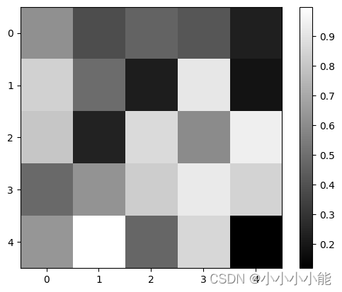
plt.imshow(rnd>0.5, cmap='gray')
plt.colorbar() 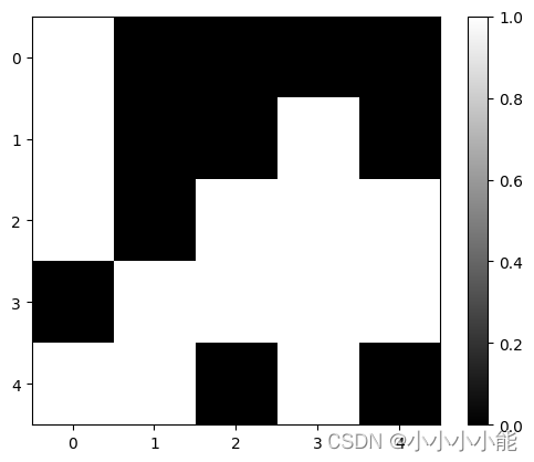
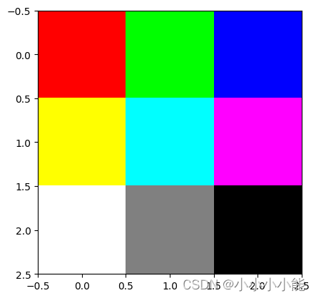
color_img = np.array([
    [[255,0,0],
     [0,255,0],
     [0,0,255]],
    [[255,255,0],
     [0,255,255],
     [255,0,255]],
    [[255,255,255],
     [128,128,128],
     [0,0,0]],
])
plt.imshow(color_img)