AIGC-understand DDPM (diffusion model) from a code perspective

I am going to learn AIGC recently, so I need to start with some basic networks, such as DDPM. This article will be from the code analysis perspective For everyone to learn and understand. DDPM (Denoising Diffusion Probabilistic Models) is a diffusion model.

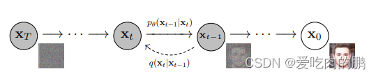
The diffusion model contains two main processes:noising processanddenoising process a>. Corresponding to the above figure, from x0 to xt is the process of adding noise, and from xt to x0 is the process of denoising.

The forward noise adding process and the reverse denoising process are bothMarkov chains, and the whole process takes about < a i=3>1000 steps.

The forward noise adding process is to continuously add noise (Gaussian noise) to the input data.

The reverse denoising process is to gradually obtain noise samples one by one from the standard Gaussian distribution, and finally obtain the generated sample data.

Among themthe noise adding process formula is:

$x_{t}=\sqrt{\alpha_{t}}x_{t-1}+\sqrt{1-\alpha _{t}}z_{1}$

Here $\sqrt{\alpha_{t}}$ is a hyperparameter set in advance, called Noise schedule, which is usually less than The value of 1 ranges from 0.9999 to 0.998. [The above formula shows how $x_{t}$ is derived from $x_{t-1}$ ].

So what is the relationship between $x_{t}$ and $x_{t-2}$ ? We can deduce it forward (that is, expand $x_{t-1}$ ):

$x_{t}=\sqrt{\alpha _{t}}(\sqrt{\alpha_{t-1}}x_{t-2}+\sqrt{1-\alpha_{t-1}}z_{2})+\sqrt{1-\alpha_{t}}z_{1}$

The noise added each time obeys the normal distribution $z_{1},z_{2}...\sim N(0,1)$ , so by sorting out the above formula, we can get:

$x_{t}=\sqrt{\alpha_{t}\alpha_{t-1}}x_{t-2}+\sqrt{1-\alpha_{t}\alpha_{t-1}}z_{2}$

Then have we found a certain pattern, and we can get the relationship between $x_{t}$ and $x_{0}$ :

$x_{t}=\sqrt{\overline{\alpha_{t}}}x_{x0}+\sqrt{1-\overline{\alpha_{t}}}z_{t}$

DDPM is defined in the code as follows:

The code uses Bubbliiing's code.

net    = GaussianDiffusion(UNet(3, self.channel), self.input_shape, 3, betas=betas)

You can see that the input parameters of the diffusion model areUNet network, and the input_shape isinput size< /span> introduced at the beginning of the article), its value is ). The definition of betas is as follows (of course you can use cosine to generate it, here I just use a linear example):What is set here is uniform distribution within 1000 (, the total number of time steps in and Noise schedule (that is, the Generate the noise table, betas is a linear timetable, which can be used for image input channel , 3 refers to the $\alpha _{t}$ schedule_lowschedule_high num_timesteps

betas = generate_linear_schedule(
                self.num_timesteps,
                self.schedule_low * 1000 / self.num_timesteps,
                self.schedule_high * 1000 / self.num_timesteps,
            )

Training forward function part

Then we go inside the code of GaussianDiffusion and look at each component. Let's go directly to the internal forward function to see how the image is processed.

    def forward(self, x, y=None):
        b, c, h, w  = x.shape
        device      = x.device

        if h != self.img_size[0]:
            raise ValueError("image height does not match diffusion parameters")
        if w != self.img_size[0]:
            raise ValueError("image width does not match diffusion parameters")
        # 随机生成batch个范围在0~1000内的数
        t = torch.randint(0, self.num_timesteps, (b,), device=device)
        return self.get_losses(x, t, y)

You can see that in the forward part of GaussianDiffusion, x is the input image, and then there is t, indicating that the random generation range is 0~num_timesteps [time step] batch_size number, or it can be understood as giving randomness to each batch (picture) Puttime stamp. Then dig into the code step by step and enter the get_losses function.

get_losses section

The following is the get_losses code, which has three inputs, x, t, y. Herex is the image we input for training, and t is the timestamp randomly generated above< a i=4>.

    def get_losses(self, x, t, y):
        # x, noise [batch_size, 3, 64, 64]
        noise           = torch.randn_like(x)  # 产生与输入图片shape一样的随机噪声(正态分布)

        perturbed_x     = self.perturb_x(x, t, noise)
        estimated_noise = self.model(perturbed_x, t, y)

        if self.loss_type == "l1":
            loss = F.l1_loss(estimated_noise, noise)
        elif self.loss_type == "l2":
            loss = F.mse_loss(estimated_noise, noise)
        return loss

Inside the function, a random noise with the same normal distribution as the size of the input image is first creatednoise, and then a>perturb_xThe function is to add noise to the input image at time t Disturbance handling.

perturb_x function part

Then let’s take a look at how perturb_x adds noise to the image at time t (keep your head clear, these codes are layered one by one like a matryoshka doll).

In this function, there are three input parameters: Enter a picture, and then t=323 at this time, then it can be understood as Add noise t to my picture when the timestamp is 323, and this picture corresponds to Input Xt at time t. sqrt_alphas_cumprod and sqrt_one_minus_alphas_cumprod use these two tensors toControl the mixing ratio of input image x and noise noise in the time dimension.

    def perturb_x(self, x, t, noise):
        '''
        :param x:输入图像
        :param t: 每个图片不同的时间戳(范围在0~1000)
        :param noise: 与输入图片shape一样的正态分布随机噪声
        :return:经过扰动后的图像
        '''
        return (
            extract(self.sqrt_alphas_cumprod, t,  x.shape) * x +
            extract(self.sqrt_one_minus_alphas_cumprod, t, x.shape) * noise
        )

We can visualize the process of perturb_x. For example, I have the following original picture without noise:

Perturb x through perturb_xThe effect after adding noise:

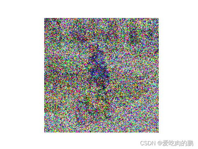
We can also control the diffusion disturbance effect of noise on the image:

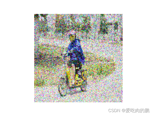
The above is the process of adding noise to the image Xt corresponding to time t. It willbecome more and more blurry as time t goes by.

Then return to the get_losses function (the code is as follows), perturbed_x is the image Xt at time t after we add noise, and the model here is our backbone networkUNetNetwork (I will take out the UNet network part separately). Then we can summarize the main process of get_losses:

Step 1.Perturb the input imagein the time domain through perturb_x, and compare it with random Noise noise is mixed, generates perturbed_x perturbed image ;

Step 2.Predict the noised image through the UNet network and obtain the predicted noise signal estimated_noise.

Step 3.Calculate the loss of predicted noise estimated_noise and real noise noise.

    def get_losses(self, x, t, y):
        # x, noise [batch_size, 3, 64, 64]
        noise           = torch.randn_like(x)  # 产生与输入图片shape一样的随机噪声(正态分布)

        perturbed_x     = self.perturb_x(x, t, noise)
        estimated_noise = self.model(perturbed_x, t, y)

        if self.loss_type == "l1":
            loss = F.l1_loss(estimated_noise, noise)
        elif self.loss_type == "l2":
            loss = F.mse_loss(estimated_noise, noise)
        return loss

That is, the Loss relationship between predicted noise and real noise is calculated during the training phase .

Prediction stage

    @torch.no_grad()
    def sample(self, batch_size, device, y=None, use_ema=True):
        if y is not None and batch_size != len(y):
            raise ValueError("sample batch size different from length of given y")

        x = torch.randn(batch_size, self.img_channels, *self.img_size, device=device)
        
        for t in tqdm(range(self.num_timesteps - 1, -1, -1), desc='remove noise....'):
            t_batch = torch.tensor([t], device=device).repeat(batch_size)
            x = self.remove_noise(x, t_batch, y, use_ema)

            if t > 0:
                x += extract(self.sigma, t_batch, x.shape) * torch.randn_like(x)
        
        return x.cpu().detach()

The prediction stage is toperform the input noise (not the input image here) Noise is processed to obtain the final generated image.

Input a normal distribution noise x, and then continuously denoise (the process of Xt~X0).

Network model structure

DDP is composed of Unet, so let’s take a look at the composition of Unet first.

class UNet(nn.Module):
    def __init__(
        self, img_channels, base_channels=128, channel_mults=(1, 2, 4, 8),
        num_res_blocks=3, time_emb_dim=128 * 4, time_emb_scale=1.0, num_classes=None, activation=SiLU(),
        dropout=0.1, attention_resolutions=(1,), norm="gn", num_groups=32, initial_pad=0,
    ):

time_mlp

self.time_mlp = nn.Sequential(
            PositionalEmbedding(base_channels, time_emb_scale),
            nn.Linear(base_channels, time_emb_dim),
            SiLU(),
            nn.Linear(time_emb_dim, time_emb_dim),
        ) if time_emb_dim is not None else None

time_mlp is composed of PositionalEmbedding layer, Linear, SiLu, and Linear.

PositionalEmbeddinglayer

class PositionalEmbedding(nn.Module):
    def __init__(self, dim, scale=1.0):
        super().__init__()
        assert dim % 2 == 0
        self.dim = dim
        self.scale = scale

    def forward(self, x):
        device      = x.device
        half_dim    = self.dim // 2
        emb = math.log(10000) / half_dim
        emb = torch.exp(torch.arange(half_dim, device=device) * -emb)
        # x * self.scale和emb外积
        emb = torch.outer(x * self.scale, emb)
        emb = torch.cat((emb.sin(), emb.cos()), dim=-1)
        return emb

The x in forward in the code istime (time axis), is not an image a>.

This function is mainly used for position encoding. The position encoding can use sine and cosine to calculate the position. The formula used is:

$PE_{pos,2i}=sin(pos/10000^{2i/d_{model}})$

$PE_{pos,2i+1}=cos(pos/10000^{2i/d_{model}})$

In positional encoding formulas, pos represents the index of each position in the sequence. For a sequence of length 4 x, each position is indexed from 0 to 3. When calculating the position encoding vector for each position, we will use this index value for calculation.

Specifically, pos in the formula represents the position index in the sequence, which is used to calculate the function parameters of sine and cosine during the calculation of the position encoding vector.

For example, when calculating the first position encoding vector of the position encoding matrix, the value of pos is 0; when calculating the second position encoding vector, < The value of a i=2> is 1, and so on. pos

For example, for example, I now have a sequence

# 设置向量的长度和位置编码的维度
vector_length = 4
embedding_dim = 4

# 生成位置编码矩阵
pos_encoding = np.zeros((vector_length, embedding_dim))

for pos in range(vector_length):
    for i in range(embedding_dim):
        if i % 2 == 0:
            pos_encoding[pos, i] = np.sin(pos / (10000 ** (2 * i / embedding_dim)))
        else:
            pos_encoding[pos, i] = np.cos(pos / (10000 ** (2 * (i - 1) / embedding_dim)))

# 打印位置编码矩阵
print(pos_encoding)

The obtained position encoding matrix is as follows

[[ 0.00000000e+00 1.00000000e+00 0.00000000e+00 1.00000000e+00]
[ 8.41470985e-01 5.40302306e-01 9.99999998e-05 9.99999995e-01]
[ 9.09297427e-01 -4.16146837e-01 1.99999999e-04 9.99999980e-01]
[ 1.41120008e-01 -9.89992497e-01 2.99999995e-04 9.99999955e-01]]

Among them, each row of the array corresponds to a position of the position encoding matrix, and the first column represents The value of the sine function at this position. The second column indicates the value of the cosine function at this position. , and so on.

That is to say, in this function, we can map the position information of the input information into high-latitude space throughsin and cos , getlocation features.

ResidualBlock

class ResidualBlock(nn.Module):
    def __init__(
        self, in_channels, out_channels, dropout, time_emb_dim=None, num_classes=None, activation=SiLU(),
        norm="gn", num_groups=32, use_attention=False,
    ):
        super().__init__()

        self.activation = activation

        self.norm_1 = get_norm(norm, in_channels, num_groups)
        self.conv_1 = nn.Conv2d(in_channels, out_channels, 3, padding=1)

        self.norm_2 = get_norm(norm, out_channels, num_groups)
        self.conv_2 = nn.Sequential(
            nn.Dropout(p=dropout), 
            nn.Conv2d(out_channels, out_channels, 3, padding=1),
        )

        self.time_bias  = nn.Linear(time_emb_dim, out_channels) if time_emb_dim is not None else None
        self.class_bias = nn.Embedding(num_classes, out_channels) if num_classes is not None else None

        self.residual_connection    = nn.Conv2d(in_channels, out_channels, 1) if in_channels != out_channels else nn.Identity()
        self.attention              = nn.Identity() if not use_attention else AttentionBlock(out_channels, norm, num_groups)
    
    def forward(self, x, time_emb=None, y=None):
        out = self.activation(self.norm_1(x))
        # 第一个卷积
        out = self.conv_1(out)
        
        # 对时间time_emb做一个全连接，施加在通道上
        if self.time_bias is not None:
            if time_emb is None:
                raise ValueError("time conditioning was specified but time_emb is not passed")
            out += self.time_bias(self.activation(time_emb))[:, :, None, None]

        # 对种类y_emb做一个全连接，施加在通道上
        if self.class_bias is not None:
            if y is None:
                raise ValueError("class conditioning was specified but y is not passed")

            out += self.class_bias(y)[:, :, None, None]

        out = self.activation(self.norm_2(out))
        # 第二个卷积+残差边
        out = self.conv_2(out) + self.residual_connection(x)
        # 最后做个Attention
        out = self.attention(out)
        return out

. . . . Not updated yet