[OpenCV image implementation: producing cool animation effects]

overview

First, by importing the necessary libraries, including NumPy for mathematical operations and the Matplotlib library for data visualization. Then, create the graph and axes, initialize the position of the points, and write the initialization and update functions.

The initialization function is responsible for setting the initial state of the graph, including the range of the coordinate axes, etc. The update function defines the change of each frame of the animation. Here, the cos function is used as an example to calculate the new coordinate position of the point.

Through the FuncAnimation class, set the animation frame number, initialization function, update function and other parameters, and finally call plt.show() to display the animation.

Generate background image

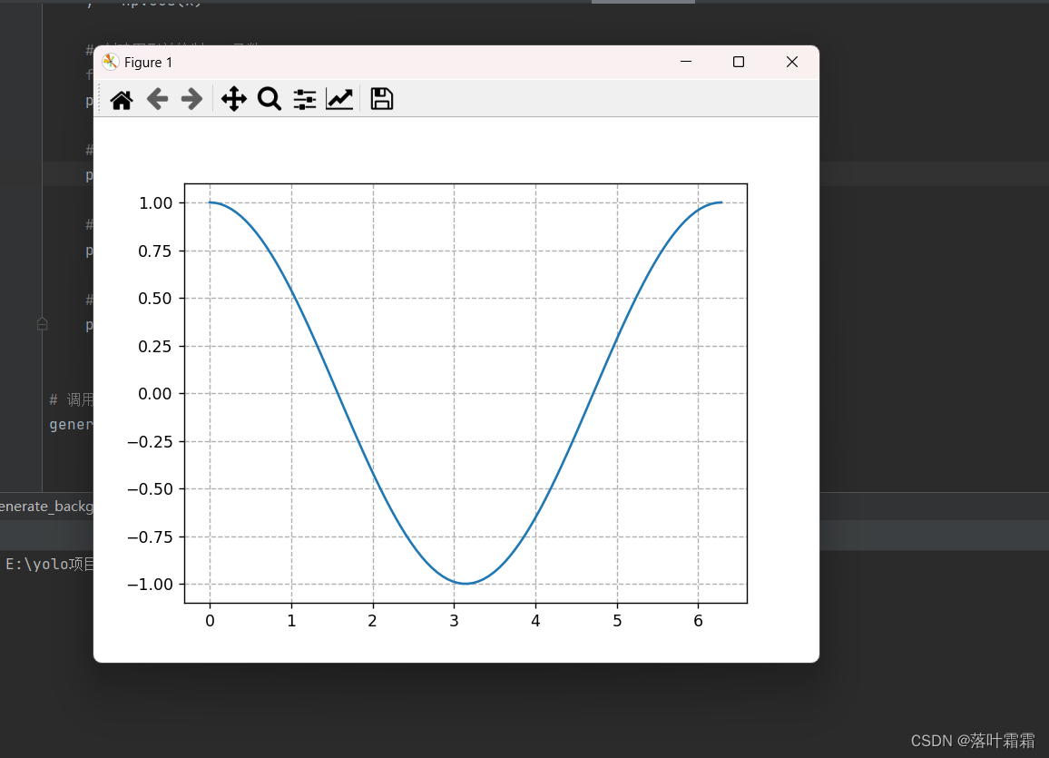
Before drawing animation, you first need to generate the background image of the cos function. This step is very simple and similar to how you normally plot with Matplotlib.

import numpy as np
import matplotlib.pyplot as plt


def generate_background():
    x = np.linspace(0, 2 * np.pi, 100)
    y = np.cos(x)

    # 创建图形并绘制cos函数
    fig = plt.figure()
    plt.plot(x, y)

    # 添加网格线
    plt.grid(ls='--')

    # 保存生成的背景图
    plt.savefig("cos_background.png")

    # 显示图形（可选）
    plt.show()


# 调用函数生成背景图
generate_background()

Add point animation

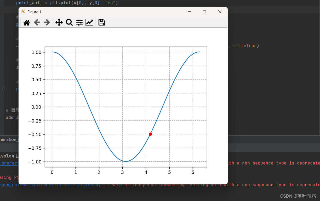
This step uses the animation library to add animation points to the code.

import numpy as np
import matplotlib.pyplot as plt
import matplotlib.animation as animation


def update_points(num):
    point_ani.set_data(x[num], y[num])
    return point_ani,


def add_animation_points():
    global point_ani, x, y
    x = np.linspace(0, 2 * np.pi, 100)
    y = np.cos(x)

    # 创建图形并绘制cos函数
    fig = plt.figure()
    plt.plot(x, y)

    # 初始化动画点
    point_ani, = plt.plot(x[0], y[0], "ro")

    # 添加网格线
    plt.grid(ls="--")

    # 创建动画
    ani = animation.FuncAnimation(fig, update_points, np.arange(0, 100), interval=100, blit=True)

    # 保存动画为gif文件
    ani.save('cos_animation.gif', writer='imagemagick', fps=10)

    # 显示动画（可选）
    plt.show()


# 调用函数添加动画点
add_animation_points()

explain:

In the above code, a function called update_points is first defined, which is used to update the data points in the plotted image. The input parameter num of the function represents the frame of the current animation, and the return value of the function is the object we need to update.

Next, pass this function into the FuncAnimation function. Its main parameters are introduced as follows:

fig: 当前绘图对象
update_points: 更新动画的函数
np.arange(0, 100): 动画帧数，这里需要是一个可以迭代的对象
interval: 动画的时间间隔
blit: 是否开启动画渲染

Finally, save the animation as a GIF file and optionally display the animation effect.

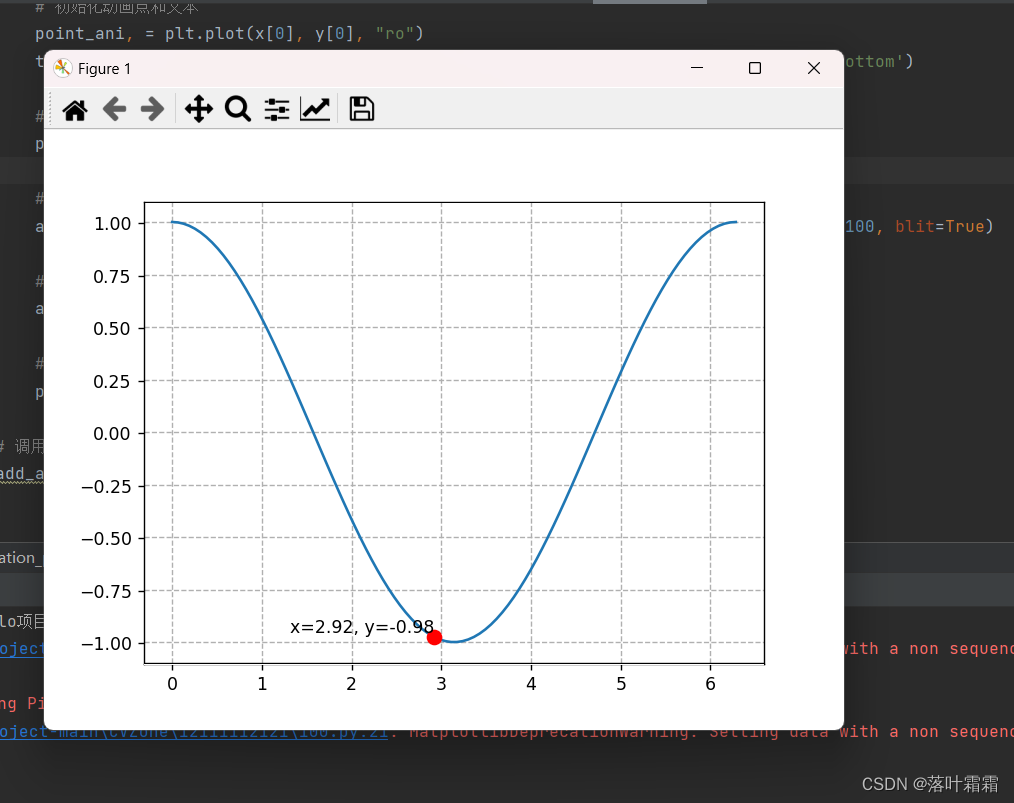
Add text display

The above code has implemented a simple point animation effect. `

The above code can be slightly modified to support the display of text and display different point styles under different conditions.

The above effect can be achieved by adding some additional code logic in the update_points function.

def update_points_v3(num):
    point_ani.set_data(x[num], y[num])
    if num % 5 == 0:
        point_ani.set_marker("*")
        point_ani.set_markersize(12)
    else:
        point_ani.set_marker("o")
        point_ani.set_markersize(8)
    text_pt.set_position((x[num], y[num]))
    text_pt.set_text("x=%.2f, y=%.2f" % (x[num], y[num]))
    return point_ani, text_pt,

Complete code:

import numpy as np
import matplotlib.pyplot as plt
import matplotlib.animation as animation

def update_points(num):
    point_ani.set_data(x[num], y[num])
    text_pt.set_position((x[num], y[num]))
    text_pt.set_text("x=%.2f, y=%.2f" % (x[num], y[num]))
    return point_ani, text_pt

def update_points_v2(num):
    # 每隔5帧改变点的样式
    if num % 5 == 0:
        point_ani.set_marker("*")
        point_ani.set_markersize(12)
    else:
        point_ani.set_marker("o")
        point_ani.set_markersize(8)

    # 更新动画点和文本显示
    point_ani.set_data(x[num], y[num])
    text_pt.set_position((x[num], y[num]))
    text_pt.set_text("x=%.2f, y=%.2f" % (x[num], y[num]))

    return point_ani, text_pt

def add_animation_points():
    global point_ani, text_pt, x, y
    x = np.linspace(0, 2 * np.pi, 100)
    y = np.cos(x)

    # 创建图形并绘制cos函数
    fig = plt.figure()
    plt.plot(x, y)

    # 初始化动画点和文本
    point_ani, = plt.plot(x[0], y[0], "ro")
    text_pt = plt.text(x[0], y[0], "x=%.2f, y=%.2f" % (x[0], y[0]), ha='right', va='bottom')

    # 添加网格线
    plt.grid(ls="--")

    # 创建动画
    ani = animation.FuncAnimation(fig, update_points_v2, np.arange(0, 100), interval=100, blit=True)

    # 保存动画为gif文件
    ani.save('cos_animation.gif', writer='imagemagick', fps=10)

    # 显示动画（可选）
    plt.show()

# 调用函数添加动画点
add_animation_points()

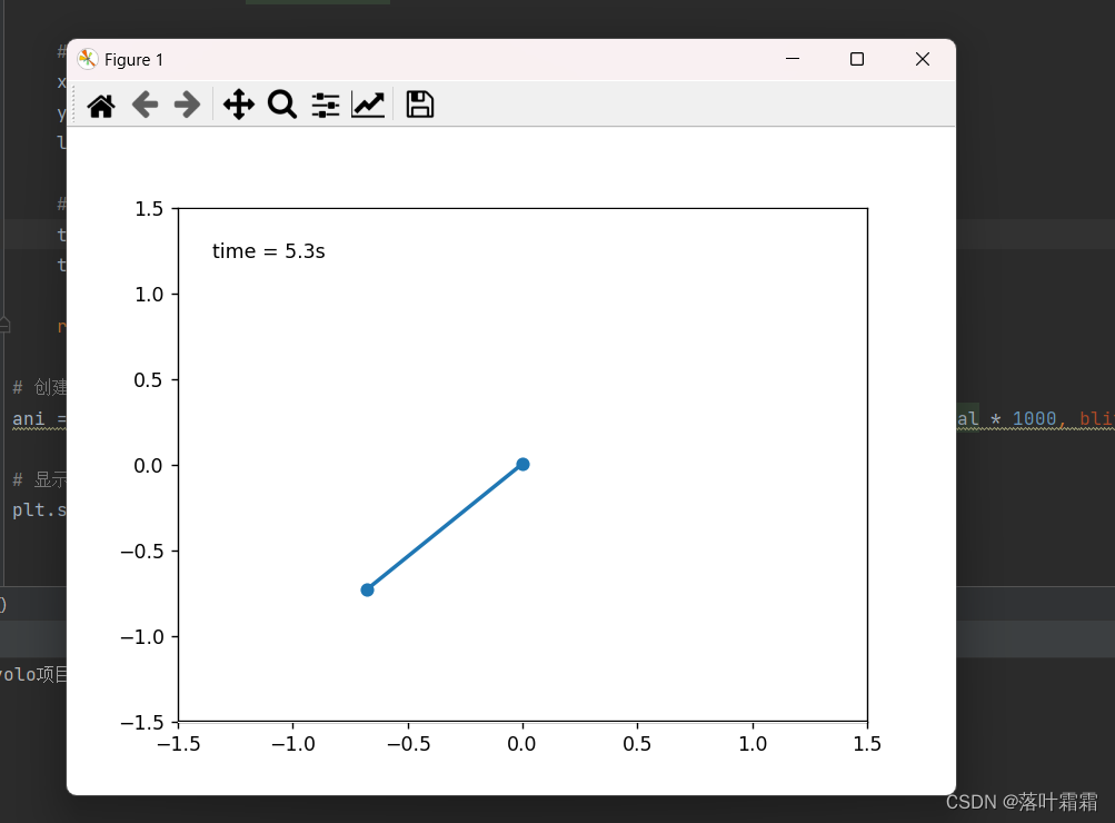
result

import numpy as np
import matplotlib.pyplot as plt
import matplotlib.animation as animation

# 定义常量
g = 9.8  # 重力加速度
length = 1.0  # 钟摆长度
theta0 = np.pi / 4.0  # 初始摆角
time_interval = 0.05  # 时间间隔

# 计算角速度
omega0 = 0.0
omega = omega0

# 初始化时间和角度
t = 0.0
theta = theta0

# 创建画布和子图
fig, ax = plt.subplots()
ax.set_xlim(-1.5, 1.5)
ax.set_ylim(-1.5, 1.5)

# 初始化绘制的对象
line, = ax.plot([], [], 'o-', lw=2)
time_template = 'time = %.1fs'
time_text = ax.text(0.05, 0.9, '', transform=ax.transAxes)

# 更新函数，用于每一帧的绘制
def update(frame):
    global theta, omega, t

    # 计算新的角度和角速度
    alpha = -g / length * np.sin(theta)
    omega += alpha * time_interval
    theta += omega * time_interval

    # 更新绘制的数据
    x = [0, length * np.sin(theta)]
    y = [0, -length * np.cos(theta)]
    line.set_data(x, y)

    # 更新时间文本
    t += time_interval
    time_text.set_text(time_template % t)

    return line, time_text

# 创建动画
ani = animation.FuncAnimation(fig, update, frames=range(0, 100), interval=time_interval * 1000, blit=True)

# 显示动画
plt.show()

summary

The cos function is explained as an example, and the animation effect of points moving along the cos curve is realized step by step
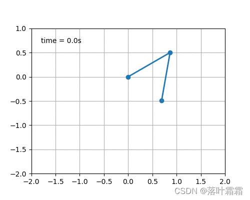
Physical model: A simple physical model is used to describe two interconnected Pendulum system. Each pendulum is affected by gravity, and the motion of the first pendulum is transferred to the second pendulum.

Mathematical Modeling: Simple physical equations, including angular velocity, angle, and Newton's equations of motion, are applied to model the motion of a pendulum.

Matplotlib's Animation class: Using Matplotlib's Animation class, the pendulum position is updated and drawn in each frame. Through scheduled updates, we get a vivid pendulum swing animation effect.

Interactive display: Using Matplotlib's plt.show() function, the animation can be displayed in real time in the graphical interface, allowing users to observe the movement of the pendulum.