0. Introduction
Generally speaking, when the system passes through irregular terrain, the robot itself will move violently, which will cause motion distortion in lidar scanning, which may reduce the accuracy of state estimation and mapping. Although some methods have been used to mitigate this effect, they are still too simple or computationally expensive to be applied to resource-constrained mobile robots. Previously, this team developed the method "Classic Literature Reading – DLO". The team proposed the article "Direct LiDAR-Inertial Odometry: Lightweight LIO with Continuous-Time Motion Correction" in 2023. This lightweight lidar inertial navigation system algorithm uses a new coarse-to-fine approach to construct continuous-time trajectories for precise motion correction. The key to this method is to construct a set of analytical equations parameterized only by time, so that the point-by-point dedistortion process can be fast and parallelizable. This approach is possible because of the strong convergence properties of our nonlinear geometric observer, which provides reliable state estimation initialization for the sensitive integration step of the IMU. Relevant code can be found on GIthub.
1. Main contributions
This paper proposes a fast and reliable odometry method called Direct LiDAR-Inertial Odometry (DLIO), which provides precise positioning and detailed 3D mapping (see Figure 1), with four main contributions.
- First, we propose a newcoarse-to-fine technique for constructing continuous-time trajectories, in which a set of Analytical equations for motion models with constant jerk and angular acceleration for fast and parallelizable point-by-point motion correction.
- Secondly, a new simplified structure is proposed to mergemotion correction and prior construction into one step and directly perform scan-to-map registration< a i=2>, which greatly reduces the overall computational load of the algorithm. (Point-LIO is also doing this work)
- Third, we exploit a new nonlinear geometric observer [10], which hasstrong performance guarantees and is crucial to achieve the first two contributions< /span>, robustly generate accurate estimates of the robot's complete state with minimal computational complexity in a pipeline.
- Finally, we demonstrate the effectiveness of our approach through extensive experimental validation of state-of-the-art techniques using multiple datasets.
2. System Overview
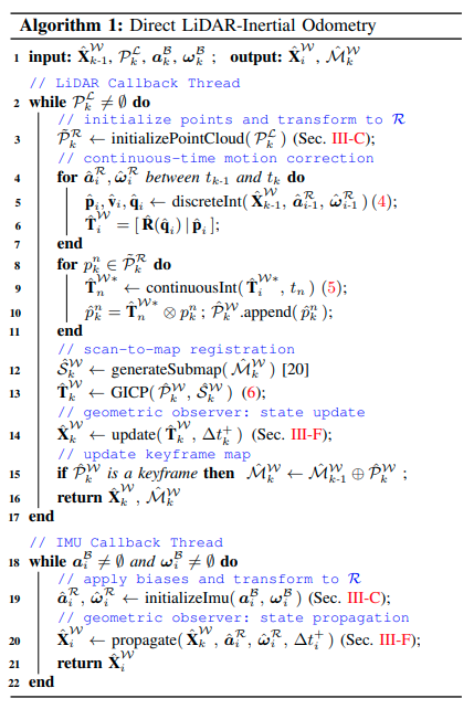
DLIO is a lightweight LIO algorithm that generates robot state estimates and geometric maps through a unique architecture containing two main components and three innovations W W with extracted local submaps. Register to the robot's map. atfast scan matcher that combines dense, motion-corrected point clouds by aligning them (see Figure 2). The first component is a Continuous time integration is performed point by point in W to ensure that the corrected point cloud has maximum image fidelity, while establishing a priori for GICP optimization. In the second component, anonlinear geometric observer [10] updates the system state using the attitude output of the first component, providing high-speed and reliable estimates of attitude, velocity, and sensor bias< /span>, these estimates have global convergence. These estimates then initialize the next iteration of motion correction, scan matching, and state updates.
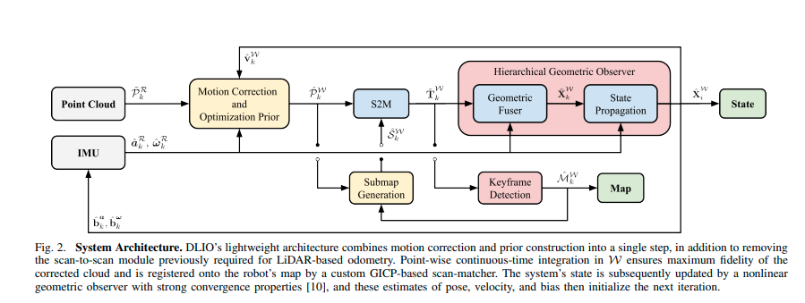
Figure 2. System architecture. DLIO’s lightweight architecture combines motion correction and prior construction into a single step and removes the scan-to-scan module previously required for lidar-based odometry. Continuous time integration is performed point by point in W, ensuring that the corrected point cloud has maximum fidelity and is registered to the robot's map via a custom GICP-based scan matcher. Subsequently, the state of the system is updated by a nonlinear geometric observer [10] with strong convergence properties, and these estimates of attitude, velocity and bias then initialize the next iteration.
3. Symbolic representation
Suppose at time t k t_k tkThe point cloud of a single lidar scan starting from is expressed as P k P_k Pk,并用 k k kProgress index. Pointyun P k P_k PkBy the time difference relative to the scan start time Δ t k n Δt^n_k ∆tkn Measurement point p k n ∈ R 3 p^n_k∈\mathbb{R}^3 pkn∈R3organization, inside n = 1 , … , N n = 1, …, N n=1,…,N, N N N is the total number of points in the scan. The world coordinate system is expressed as W W W, the robot coordinate system is expressed as R R R, the center of gravity, the middle x x xdirection forward, y y yoriented left, z z z points upward. The coordinate system of IMU is expressed as B B B, the coordinate system of lidar is expressed as L L L, Equipment presence index k k State vector at k X k X_k XkDefined as a tuple.
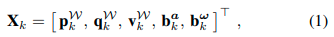
Naka p W ∈ R 3 p^W ∈ \mathbb{R}^3 pIN∈R3 is the position of the robot, q W q^W qW is the direction of quaternion encoding, expressed in Hamilton notation, located at S 3 \mathbb{S}^3 S3, v W ∈ R 3 v^W ∈\mathbb{R}^3 inIN∈R3This is mechanical speed, b a ∈ R 3 b^a ∈ \mathbb{R}^3 ba∈R3 is the bias of the accelerometer, b ω ∈ R 3 b^ω ∈ \mathbb{R}^3 boh∈R3 is the deviation of the gyroscope. Measured value of IMU a ^ \hat{a} a^和 ω ^ \hat{ω} oh^Construction model
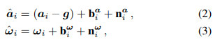
并用 i = 1 , … , M i = 1, …, M i=1,…, M is indexed, indicating that at clock time t k − 1 t_{k-1} tk−1和 t k t_k tk之间 M M M measurements. For simplicity, unless otherwise stated, indexes k k k sum i i i appears on lidar and IMU rates respectively, and is written in this way . Raw sensor measurements a i a_i aisum ω i ω_i ohiInclusion deviation b i b_i biJapanese rant n i n_i ni, g g g is the gravity vector after rotation. In this paper, we address the following problem: Given a cumulative point cloud from lidar P k P_k Pk and measurements sampled by the IMU between each scan received a i a_i ai **sum ** ω i ω_i ohi, estimate the state of the robot X ^ i W \hat{X}^W_i X^iWAnd geometric map M ^ k W \hat{M}^W_k M^kW。
4. Preprocessing
The input to DLIO is a dense 3D point cloud collected by a 360-degree mechanical LiDAR such as Ouster or Velodyne (10-20Hz), and time-synchronized linear acceleration and angular velocity measurements from a 6-axis IMU, IMU rate Much higher than radar (100-500Hz). Prior to downstream tasks, all sensor data are converted via external calibration to R R located at the robot's center of gravityR. For IMU, the effect of measuring displacement by linear acceleration on a rigid body must be considered. If the sensor does not coincide with the center of gravity, then by considering all linear accelerations in < /span> R R R is accomplished by the cross product between angular velocity and IMU offset. To minimize information loss, in addition to using 1 m 3 1m^3 1mIn addition to a box filter of 3 to remove points that may come from the robot itself, and a lightweight voxel filter for higher resolution point cloud processing, we do not Point clouds are preprocessed. This distinguishes our work from other work that attempts to detect features (such as corners, edges or surfels) or heavily downsample clouds through voxel filters.
5. Continuous-time motion correction with joint prior (key content)
The point cloud collected by the rotating LiDAR sensor will be affected by motion distortion during movement because the rotating laser array collects points at different times during the scanning process. We no longer assume simple motion (e.g., constant velocity) to capture fine motion, but instead use more accurate constant acceleration and angular acceleration models via a two-step coarse-to-fine propagation scheme as Compute a unique transformation for each point. This strategy aims to minimize errors due to the IMU's sampling rate and the time offset between the IMU and LiDAR point measurements. The scanned trajectory is first roughly constructed via numerical IMU integration in W [29] and subsequently refined by solving a set of analytical continuous-time equations (Fig. 3).
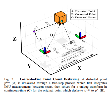
Figure 3. Coarse-to-fine point cloud dedistortion. De-distort the distorted points through a two-step process p L 0 ( A ) p^{L_0}(A) pL0(A), first integrating the IMU measurements between scans, then in continuous time Solve the unique transformation (C) to transform the original point p L 0 p^{L_0} pL0Elimination change p ∗ p^∗ p∗(B)
ប្រំា t k t_k tk is received with N N NCumulative points P k R P^R_k PkRclock time of , and t k + Δ t k n t_k + Δt^n_k tk+∆tknis the center point of the cloud p k n p^n_k pknThe timestamp of . To approximate each point at W W For the position in W, we first determine the position in t k − 1 t_{k-1} tk−1和 t k + ∆ t k N t_k + ∆t^N_k tk+∆tkNIntegrate IMU measurements between to obtain a motion estimate:

对于 i = 1 , … , M i = 1, …, M i=1,…, M, inside M M M is the number of IMU measurements between two scans, where j ^ i = 1 Δ t i ( R ^ ( q ^ i ) a ^ i − R ^ ( q ^ i − 1 ) a ^ i − 1 ) \hat{j}_i = \frac{1}{Δt_i}(\hat{R}(\hat{q}_i) \hat{a}_i - \hat{R}(\hat{q}_{i-1})\hat{a}_{i-1}) j^i=∆ti1(R^(q^i)a^i−R^(q^i−1)a^i−1), α ^ i = 1 ∆ t i ( ω ^ i − ω ^ i − 1 ) \hat{α}_i = \frac{1}{∆t_i}(\hat{ω}_i - \hat{ω}_{i-1}) a^i=∆ti1(oh^i−oh^i−1)separationis the calculated linear jerk sum angular acceleration. Give p ^ i \hat{p}_i p^i和 q ^ i \hat{q}_i q^iCorresponding set of homogeneous transformations T ^ i W ∈ S E (3) \hat{T}^W_i∈\mathbb{SE} (3) T^iW∈SE(3)ThenDefines a coarse discrete-time trajectory during the scan. Then, transform from the nearest predecessor to each point p k n p^n_k pknAnalytical continuous-time solution of recovers point-specific dedistortion transformations T ^ n W ∗ \hat{T}^{W∗}_n T^nW∗, making
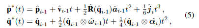
In that, i − 1 i-1 i−1sum i i i corresponds to the latest previous and next IMU measurements respectively, t t tKore point p k n p^n_k pknTimestamp between and the most recent previous IMU, T ^ n W ∗ \hat{T}^{W∗}_n T^nW∗は对于 p k n p^n_k pkn corresponds to p ∗ p^∗ p∗和 q ∗ q^∗ qTransformation of ∗ (Figure 4). Note that (5) is only given by t t t is parameterized so that any desired time transformation can be queried to construct continuous-time trajectories.