1, data0507 flower is the flowering height of a certain plant at two altitudes and two temperatures. Use appropriate statistical methods to test the flowering height of this plant at different temperatures. Are there any differences between altitudes and temperatures? If there is a difference, how is it different? (Explain key information such as basis and conclusion, including key information involved in the calculation process)
library(HH) #interaction2wt() in the HH package can display main effects and interaction effects at the same time
flower <- read.delim("D:/Datum/Biostatistics/data/data5/data0507 flower.txt")
flower
   Altitude Temperatyre Height
1         1           1  148.7
2         1           1  148.3
3         1           1  147.7
4         1           1  148.7
5         1           1  148.3
6         1           1  147.7
7         1           1  148.7
8         1           1  148.3
9         1           1  147.7
10        1           1  143.0
11        1           1  142.7
12        1           1  142.0
13        1           1  143.0
14        1           1  142.7
15        1           1  142.0
16        1           1  143.0
17        1           1  142.7
18        1           1  142.0
19        1           1  150.3
20        1           1  149.3
21        1           1  148.7
22        1           1  150.3
23        1           1  149.3
24        1           1  148.7
25        1           1  149.3
26        1           1  149.3
27        1           1  149.0
28        2           1  135.3
29        2           1  136.0
30        2           1  135.7
31        2           1  135.3
32        2           1  135.7
33        2           1  133.0
34        2           1  134.0
35        2           1  133.7
36        2           1  133.0
37        2           1  134.0
38        2           1  133.7
39        2           1  149.3
40        2           1  149.0
41        2           1  149.3
42        2           1  135.3
43        2           1  135.7
44        2           1  135.3
45        2           1  139.3
46        2           1  139.7
47        2           1  138.7
48        1           2  135.3
49        1           2  136.0
50        1           2  135.7
51        1           2  133.0
52        1           2  134.0
53        1           2  133.7
54        1           2  135.3
55        1           2  135.7
56        1           2  135.3
57        1           2  135.3
58        1           2  135.7
59        1           2  135.3
60        1           2  135.7
61        1           2  136.0
62        1           2  135.3
63        1           2  134.3
64        1           2  134.3
65        2           2  135.3
66        2           2  135.7
67        2           2  135.3
68        2           2  135.7
69        2           2  130.7
70        2           2  133.3
71        2           2  133.7
72        2           2  130.7
73        2           2  133.3
74        2           2  133.7
75        2           2  130.7
76        2           2  133.3
77        2           2  133.0
78        2           2  133.3
79        2           2  136.0
80        2           2  136.0
81        2           2  133.3
82        2           2  136.0
83        2           2  136.0
84        2           2  133.3
85        2           2  136.0
86        2           2  136.0
87        2           2  142.3
str(flower) # View data structure
summary(flower) # View data summary statistics
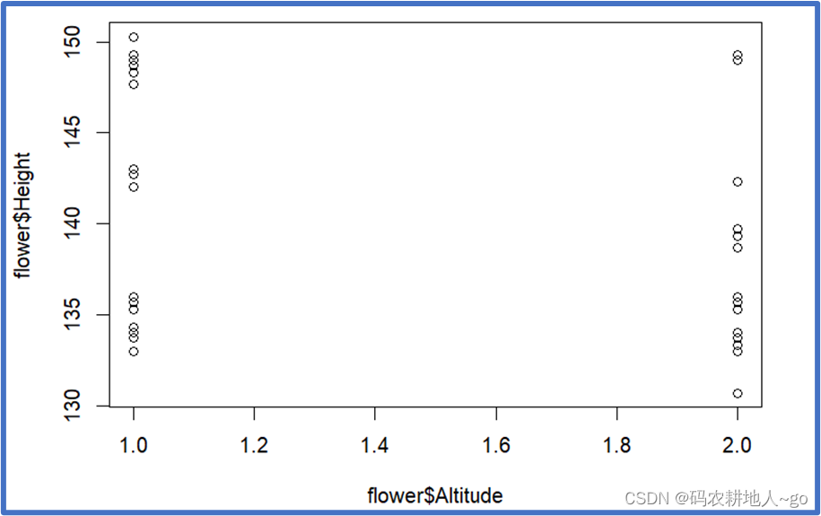
plot(flower$Altitude, flower$Height) # Draw a scatter plot of altitude and flowering height
plot(flower$Temperatyre, flower$Height) # Draw a scatter plot of temperature and flowering height
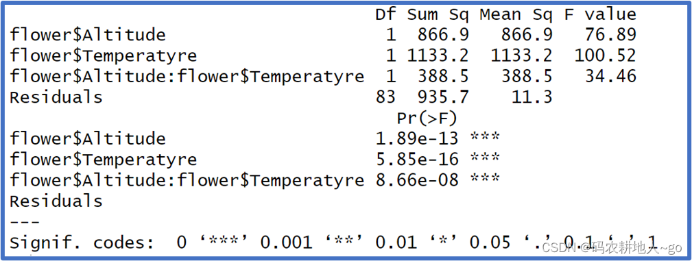
summary(aov(flower$Height~flower$Altitude*flower$Temperatyre))
#For the flowering height of this plant, there is an interaction between altitude and temperature (F1,83=34.46, P<0.001)
#After controlling the interaction between altitude and temperature that affects flowering height, the flowering height of this plant has extremely significant differences between different altitudes (F1, 83 =76.89, P<0.001)
#After controlling the interaction between altitude and temperature that affects flowering height, the flowering height of this plant has extremely significant differences between different temperatures (F1, 83 =100.52, less than 0.001)
interaction2wt(flower$Height~flower$Altitude*flower$Temperatyre) #Show main effect and interaction effect
#The higher the temperature [from 1 to 2], the lower the flowering height
#The higher the altitude [from 1 to 2], the lower the flowering height


2, data0508 develop is the growth period of three insects under seven conditions. Appropriate statistical methods are used to test the growth period between different species and different conditions. Is there any difference between them? If there is a difference, how is it different? (Explain key information such as basis and conclusion, including key information involved in the calculation process)
library(HH) #interaction2wt() in the HH package can display main effects and interaction effects at the same time
develop <- read.delim("D:/Datum/biostatistics/data/data5/data0508 develop.txt")
develop
   Species Condition  Day
1        1         1  9.6
2        1         2 10.6
3        1         3  9.8
4        1         4 10.7
5        1         5 11.1
6        1         6 10.9
7        1         7 12.8
8        2         1  9.3
9        2         2  9.1
10       2         3  9.3
11       2         4  9.1
12       2         5 11.1
13       2         6 11.8
14       2         7 10.6
15       3         1  9.3
16       3         2  9.2
17       3         3  9.5
18       3         4 10.0
19       3         5 10.4
20       3         6 10.8
21       3         7 10.7
str(develop) # View data structure
summary(develop) #View data summary statistics
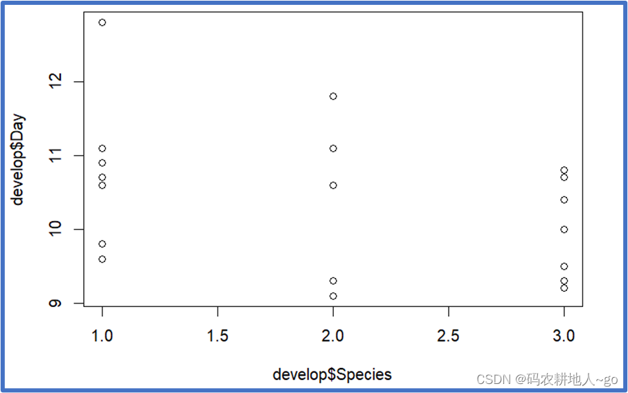
plot(develop$Species, develop$Day) # Draw a scatter plot of three species and insect growth stages
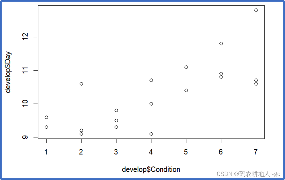
plot(develop$Condition, develop$Day) # Draw a scatter plot of seven conditions and flowering height
# two fixed factors, full model
summary(aov(develop$Day~develop$Species*develop$Condition))
There is no interaction
# two fixed factors, no interaction
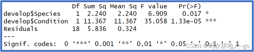
summary(aov(develop$Day~develop$Species+develop$Condition))
#After controlling for the influence of conditions, there are significant differences in the growth stages of different insects (P=0.017, less than 0.05)
#After controlling for the influence of insect species, there are extremely significant differences in the measured growth periods of insects under different conditions (P=1.33e-05, less than 0.001)< /span>
# two fixed factors, full model
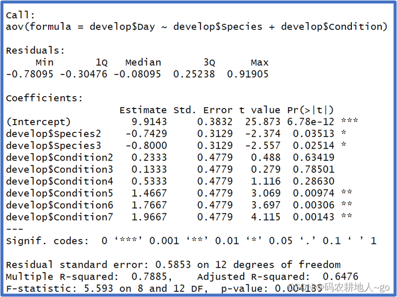
summary.lm(aov(develop$Day~develop$Species+develop$Condition))
#For species effects (Species), species B and species C have more significant negative effects, that is, species B and species C have a shorter growth period,
#ConditonC5, ConditonC6, and ConditonC7 have a significant positive effect on condition (Condition), that is, ConditonC5, ConditonC6, and ConditonC7 have a longer growth period
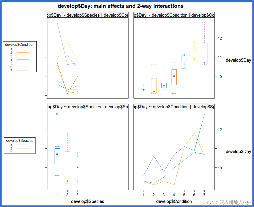
interaction2wt(develop$Day~develop$Species+develop$Condition) #View the main effect
#Growth: Species A>B>C (based on the results in the lower left corner and summary.lm)
#Growth: Condition 7>6>5>4>2>3>1 (based on the results in the upper right corner and summary.lm)