Performance Engineering for Language Large Model Inference: Best Practices

In this post, the MosaicML engineering team shares best practices for how to make the most of popular open source language large models (LLMs) in production environments. Additionally, they provide guidance on deploying inference services around models to help users better select models and deploy hardware. They use multiple PyTorch-based backends in production. These guidelines are summarized by the MosaicML engineering team based on the experience behind FasterTransformers, vLLM, and NVIDIA's TensorRT-LLM.

MosaicML open sourced the MPT-7B and MPT-30B language large models in the middle of this year, and was subsequently acquired by Databricks for US$1.3 billion.

(The following content is compiled and published by OneFlow. Please contact us for authorization for reprinting. Original text: https://www.databricks.com/blog/llm-inference-performance-engineering-best-practices)

Source | Databricks

OneFlow compilation

Translation｜Yang Ting, Wan Zilin

Understanding text generation from large language models

Text generation for large language models can usually be divided into two stages: first, the "prefill" stage, which processes the tokens in the input prompt in parallel; then, the "decoding" stage, At this stage, the text generates "word elements" one by one in an autoregressive manner. Each generated token is added to the input and re-fed to the model to generate the next token. The generation process stops when the LLM outputs a special stop token or when user-defined conditions are met (such as the maximum number of tokens generated).

Tokens can be words or subwords, and the exact rules for splitting text into tokens vary from model to model. For example, we can compare the way the LLaMA model and the OpenAI model segment text. Although LLM inference service providers often talk about performance in terms of token-based metrics (such as tokens processed per second), these numbers are not always comparable between different model types due to differences in model tokenization rules. . For example, the Anyscale team found that LLaMA 2's word segmentation length increased by 19% compared to ChatGPT's word segmentation length (but the overall cost was much lower). Researchers at HuggingFace also found that compared with GPT-4, for the same length of text, LLaMA 2 training requires about 20% more tokens.

LLMImportant indicators of services

How should we accurately measure the inference speed of a model?

Our team uses the following four metrics:

Time To First Token (TTFT): This is the time it takes for the model to generate the first output after the user inputs the query. Getting responses with low latency is important in real-time interactions, but less so in offline workloads. This metric is driven by the time it takes to process the hint and generate the first output token.
Time Per Output Token (TPOT): The time required to generate an output token for each user querying the system. This metric is related to each user's perception of the "speed" of the model. For example, a TPOT of 100 milliseconds/word means that each user can process 10 words per second, or about 450 words per minute, which is far faster than the reading speed of ordinary people.
Latency: The total time it takes for the model to generate a complete response for the user. The overall response delay can be calculated using the first two indicators: delay = (TTFT) + (TPOT) * (number of tokens to be generated ).
Throughput: The number of output tokens the inference server can generate per second across all users and requests.

Our goals are:Generate the first token in the shortest time, achieve the highest throughput, and generate the output token in the shortest time. In other words, we want the model to be able to generate text for as many users as quickly as possible.

It is worth noting that we need to trade off throughput and time per output token: compared to running the queries sequentially, if we process 16 user queries simultaneously, the throughput will be higher, but it will take longer to process each output token. A user generates output tokens.

If you have specific goals for overall inference latency, here are some effective heuristics for evaluating your model:

Output length determines overall response latency: for average latency, usually just multiply the expected/maximum output token length by the model's overall average time per output token.
Input length has little impact on performance, but is critical on hardware requirements: in the MPT model, adding 512 input tokens adds less latency than generating 8 additional output tokens. However, the need to support long inputs can make models difficult to deploy. For example, we recommend using the A100-80GB (or newer) to deploy the MPT-7B model for a maximum context length of 2048 tokens.
Overall latency scales sublinearly with model size: larger models are slower on the same hardware, but the speed ratio does not necessarily match the parameter number ratio. The latency of MPT-30B is approximately 2.5 times that of MPT-7B, and the latency of LLaMA2-70B is approximately twice that of LLaMA2-13B.

We are often asked by potential customers to provide average inference latency. In this regard, we recommend that before anchoring a specific latency goal (for example, "single token generation time is less than 20 milliseconds"), you should take some time to describe your expected input length and desired output length.

Challenges faced by large model reasoning in language

The following general techniques can be used to optimize inference for large models of language:

Operator fusion: Merging different adjacent operators together usually results in shorter latency.
Quantization: Compress activations and weights to use fewer bits.
Compression: sparsity or distillation.
Parallelization: Tensor parallelism across multiple devices, or pipeline parallelism for larger models.

In addition to the above methods, there are many important optimization techniques for Transformer, such as KV (key-value) cache. In Transformer-based decoder-only models, the attention mechanism is computationally less efficient. Each token has to pay attention to all the previously generated tokens, so every time a new token is generated, many of the same values have to be recalculated. For example, when generating the Nth word element, the (N-1)th word element should focus on the (N-2)th word element, (N-3) word element... until the 1st word element. Similarly, when (N+1) tokens are generated, the attention mechanism of the Nth token needs to pay attention to the (N-1)th, (N-2), (N-3)... until The 1st word element. The KV cache is used to save the intermediate keys/values of the attention layer for subsequent reuse to avoid repeated calculations.

Memory bandwidth is key

In LLM, computations are dominated by matrix multiplication computations; these smaller-dimensional computations are typically limited by memory bandwidth on most hardware. When generating tokens in an autoregressive manner, one of the dimensions of the activation matrix (defined by the batch size and the number of tokens in the sequence) is smaller at small batch sizes. Therefore, speed is determined by how quickly we can load model parameters from GPU memory into local caches/registers, not by how quickly the computation loads the data. The memory bandwidth available and achievable in the inference hardware is a better predictor of token generation speed than peak computational performance.

Inference hardware utilization is very important for service cost. Since GPUs are so expensive, we need to get them to do as much work as possible. Shared inference services reduce costs by combining workloads from multiple users, filling their gaps, and batching overlapping requests. For large models such as LLaMA2-70B, better price/performance is only achieved with larger batch sizes. Having an inference serving system that can run with larger batch sizes is critical for cost efficiency. However, larger batch sizes mean larger KV caches, which in turn increases the number of GPUs required to deploy the model. We need to play a game between the two and make trade-offs. Shared service operators need to weigh costs and optimize the system.

Model Bandwidth Utilization (MBU)

How optimized is the LLM inference server?

As briefly explained before, for LLM to perform inference at smaller batch sizes, especially in the decoding stage, its performance is limited by the speed of loading model parameters from device memory to the computing unit. Memory bandwidth determines the speed of data transfer. To measure underlying hardware utilization, we introduce a new metric called Model Bandwidth Utilization (MBU). The calculation formula of MBU is (actual memory bandwidth) / (peak memory bandwidth), where the actual memory bandwidth is ((total model parameter size + KV cache size) / TPOT).

For example, if a 16-bit precision model consists of 7 billion parameters and has a TPOT of 14 milliseconds, it transfers 14GB of parameters in 14 milliseconds, which means that its bandwidth usage is 1TB/second. If the peak bandwidth of the machine is 2TB/second, we are running at 50% of the MBU.

For simplicity, this example ignores the KV cache size, which is also smaller at smaller batch sizes and shorter sequence lengths. An MBU value close to 100% means that the inference system efficiently utilizes the available memory bandwidth. MBU can also be used to compare different inference systems (hardware + software) in a standardized way. MBU is complementary to model FLOPs utilization (MFU, a metric introduced by the PaLM paper), which is very important in computationally constrained situations.

Figure 1 shows the MBU in a roofline plot-like manner, with the solid diagonal line in the orange shaded area representing the maximum possible throughput at 100% saturation of the memory bandwidth. However, in real-life situations, for small batch sizes (white points), the observed performance is lower than the maximum throughput, and the degree of degradation can be measured in MBUs. For large batches (yellow area), the system is computationally limited, and the actual throughput is measured in MFU relative to the theoretical maximum throughput.

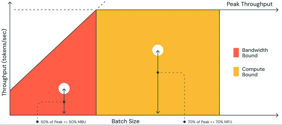
Figure 1: Shows MBU (Model Bandwidth Utilization) and MFU (Model FLOPs Utilization). MBU is the peak fraction achieved in the memory-constrained region, and MFU is the peak fraction achieved in the computation-constrained region.

MBU and MFU determine the available headroom to advance inference speed on a given hardware setup. Figure 2 shows the MBU of different tensor parallelism measured using the TensorRT-LLM based inference server. Memory bandwidth utilization reaches its peak when transferring large contiguous memory blocks. When smaller models such as the MPT-7B are distributed across multiple GPUs, we observe lower MBUs because we transfer smaller memory blocks in each GPU.

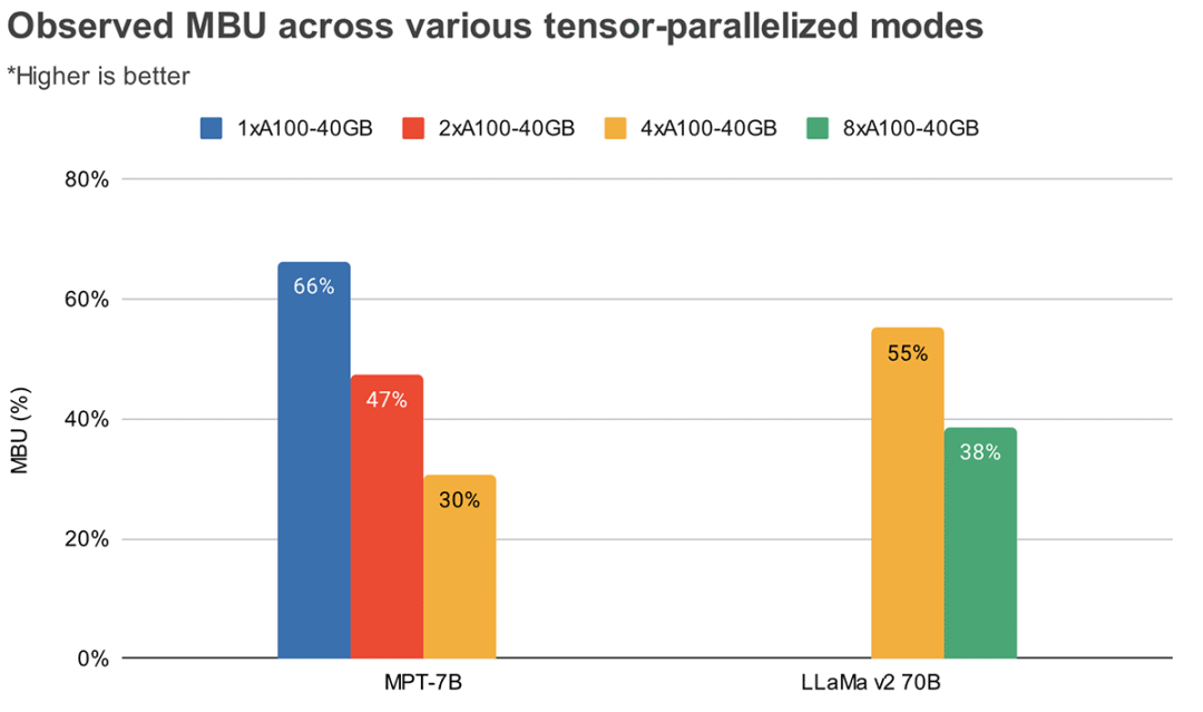
Figure 2: Empirically observed MBUs for different degrees of tensor parallelism using TensorRT-LLM on the A100-40G GPU. Request: 512 input token sequences, batch size 1.

Figure 3 shows the empirically observed MBU at different levels of tensor parallelism and batch size on an NVIDIA H100 GPU. MBU decreases as batch size increases. However, as the GPU scales, the reduction in MBU is relatively less significant. It's worth noting that hardware with greater memory bandwidth can improve performance by utilizing fewer GPUs. With a batch size of 1, we can achieve a higher MBU on 2 H100-80GB GPUs (55% MBU on the former and 55% MBU on the latter) compared to 4 A100-40GB GPUs (Figure 2) is 60%).

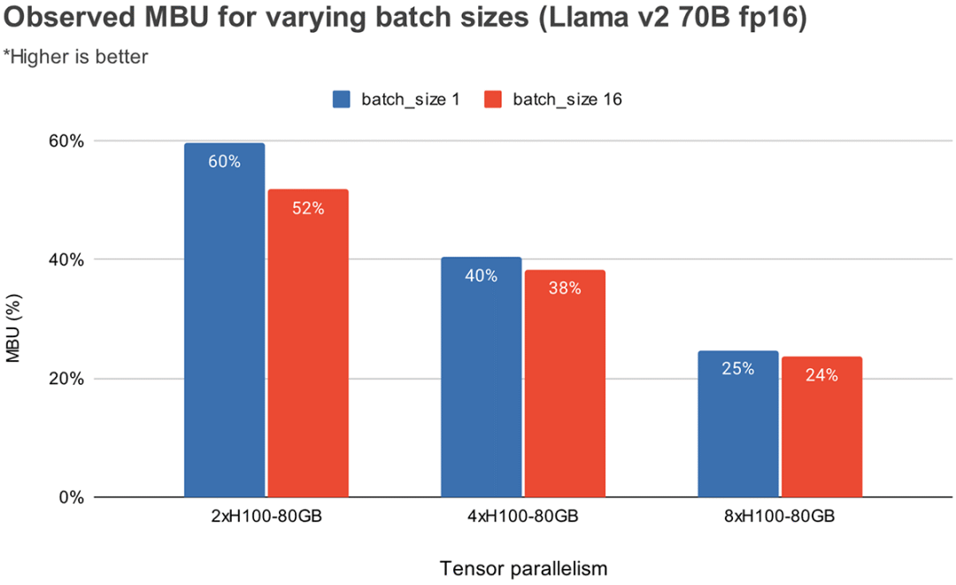
Figure 3: Empirically observed MBU for different batch sizes and tensor parallel modes on H100-80G GPU. Request: A sequence containing 512 input tokens.

Benchmark results

Delay

We measured the time to first word generation (TTFT) and the time to single output word (TPOT) under different tensor parallelism of the MPT-7B and LLaMA2-70B models. As the length of the input prompt increases, the generation time of the first token begins to account for a large portion of the overall latency. This latency can be reduced by running tensor parallelism on multiple GPUs.

Unlike model training, the gains in inference latency decrease significantly when scaling to more GPUs. For example, for the LLaMA2-70B model, scaling from 4 GPUs to 8 GPUs only reduces latency by 0.7x at smaller batch sizes. One reason is that higher parallelism results in lower MBU (as mentioned earlier). Another reason is that tensor parallelism introduces communication computational overhead between GPU nodes.

Table 1: Time required to generate the first token after inputting a request, for a length of 512 tokens and a batch size of 1. Larger models like the LLaMA2 70B require at least 4 A100-40B GPUs to match the memory.

The higher tensor parallelism results in a more significant relative reduction in token latency for larger batch sizes. Figure 4 shows the temporal changes of a single output word element in the MPT-7B model. When the batch size is 1, increasing the parallelism from 2 times to 4 times only reduces the word delay by about 12%. When the batch size is 16, the latency of 4x parallelism is reduced by 33% compared to 2x parallelism. This is consistent with our previous observation that higher tensor parallelism with a batch size of 16 results in a smaller relative reduction in MBU compared to a batch size of 1.

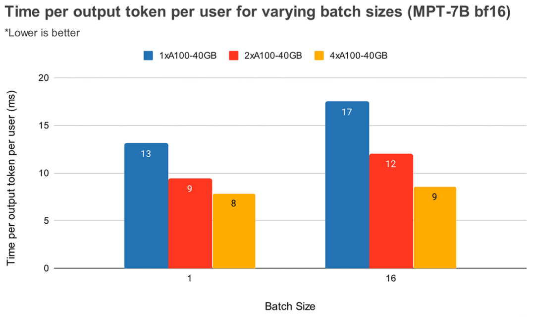
Figure 4: As we scale the MPT-7B model on A100-40GB GPUs, the latency of a single output token per user does not scale linearly with the number of GPUs. The requested token sequence includes 128 input tokens and 64 output tokens.

Figure 5 shows similar results for LLaMA2-70B, except that the relative improvement between 4x and 8x parallelism is less significant. We also compared the effects of GPU scaling on two different hardware. Since the GPU memory bandwidth of H100-80GB is 2.15 times that of A100-40GB, we can see that when the batch size is 1, the latency of the 4x parallel system is reduced by 36%, and when the batch size is 16, the latency Reduced by 52%.

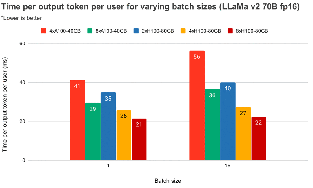
Figure 5: Time for a single output token per user as we scale the LLaMA-v2-70B model across multiple GPUs (input request: 512 token length). Please note that since LLaMA-v2-70B (using float16) cannot accommodate 1x40GB GPU, 2x40GB GPU and 1x80GB GPU systems, the data for the above systems is missing here.

Throughput

By batching requests, we can trade off throughput versus time per token. During GPU evaluation, grouping queries can increase throughput compared to processing queries one by one sequentially, but each query will take longer to complete (ignoring queuing effects).

Several common batch inference request techniques are as follows:

Static batch processing: The client packages multiple prompts into a request, and returns a response after all sequences in the batch are completed. Our inference server supports this approach but is not required to use it.
Dynamic batch processing: Dynamic batch processing will be prompted within the server. Typically this approach does not perform as well as static batching, but can get close to optimal performance if responses are short or consistent in length. Doesn't work well when requests have different parameters.
Continuous batch processing: this excellent paper (https://www.usenix.org/conference/osdi22/presentation/yu ) proposed the idea of batching requests together as they arrive, which is the current SOTA approach. Instead of waiting for all sequences in the batch to complete, it groups sequences at the iteration level. It can achieve 10x to 20x higher throughput than dynamic batch processing.

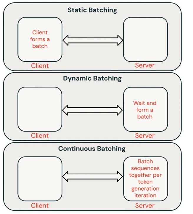
Figure 6: Different batch processing types in LLM service. Batch processing is an effective way to improve inference efficiency.

batch size

The effectiveness of batch processing depends heavily on the request stream. But by benchmarking static batching with unified requests, we can get an upper bound on its performance.

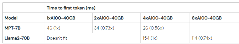
Table 2: Peak throughput (req/sec) of MPT-7B based on static batching and FasterTransformers based backend. Request: 512 input tokens and 64 output tokens. For larger inputs, the memory overflow boundary will appear at smaller batch sizes.

Latency trade-off

As batch size increases, request latency also increases. Taking an NVIDIA A100 GPU as an example, if we choose a batch size of 64 to maximize throughput, the latency will increase by 4 times, and the throughput will increase by 14 times. Shared inference services typically choose a balanced batch size. Users of the self-hosted model should decide the appropriate latency/throughput trade-off based on their application. In some applications, such as chatbots, low latency for fast responses is a primary consideration. In other applications, such as batch processing of unstructured PDFs, the latency of a single document may be sacrificed in order to process all documents quickly in parallel.

Figure 7 shows the throughput and delay curve of the 7B model. Each curve represents the results obtained by increasing the batch size from 1 to 256, which is useful for determining how large the batch size can be set under different latency constraints. Looking back at the roofline diagram above, we see that these measurements are consistent with expectations. After reaching a certain batch size, that is, when we enter the computational limit phase, each doubling of the batch size will only increase latency without increasing throughput.

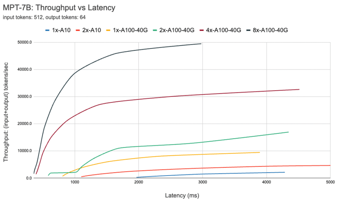
Figure 7: Throughput delay curve of MPT-7B model. This allows users to select hardware configurations that match their latency requirements to meet their throughput needs.

When using parallel computing, it is important to understand the underlying hardware details. For example, not all 8xA100 instances are the same on different cloud platforms. Some servers have high-bandwidth connections between all GPUs, while other servers pair GPUs in pairs and have lower-bandwidth connections between pairs of GPUs. This may introduce performance bottlenecks, causing actual performance to deviate significantly from the above curve.

Optimization Case Study: Quantification

Quantization is a common technique used to reduce the hardware requirements of LLM inference. Reducing model weights and activation precision during inference can significantly reduce hardware requirements. For example, reducing weights from 16 bits to 8 bits can reduce the number of GPUs required in memory-constrained environments such as the LLaMA2-70B on the A100 by half. Reducing the weight to 4 bits makes it possible for users to perform inference on consumer-grade hardware (such as LLaMA2-70B on Macbook).

In our experience, quantitative techniques should be used with caution. Simple and crude quantification techniques may lead to significant degradation in model quality, and the impact of quantification will also vary depending on the model architecture (such as MPT and LLaMA) and scale.

When experimenting with techniques such as quantification, we recommend using an LLM quality benchmark like Mosaic Eval Gauntlet to evaluate the quality of the inference system, rather than just the quality of the model alone. Additionally, it is important to explore deeper system optimizations. Specifically, quantization can make the KV cache more efficient.

As mentioned before, in autoregressive token generation, past keys/values (KVs) obtained through the attention layer are cached instead of being recomputed at each step. The size of the KV cache depends on the number of sequences processed at a time and the length of those sequences. Additionally, on each iteration that generates the next token, new KV items are added to the existing cache, and the cache becomes larger as new tokens are generated. Therefore, efficient KV cache memory management is crucial for good inference performance when adding these new values. The LLaMA2 model uses a variant called Grouped Query Attention (GQA). Note that when the number of KV heads is 1, GQA is the same as Multi-Query Attention (MQA). GQA helps reduce the size of the KV cache by sharing keys/values. The calculation formula of KV cache is:

batch_size * seqlen * (d_model/n_heads) * n_layers * 2 (K and V) * 2 (bytes per Float16) * n_kv_heads

Table 3 shows the calculated GQA KV cache size under different batch sizes with a sequence length of 1024 tokens. In comparison, the parameter size of the LLaMA2 model (70B) is 140GB (Float16). Quantizing the KV cache is a technique to reduce the size of the KV cache (in addition to GQA/MQA), and we are actively evaluating its impact on build quality.

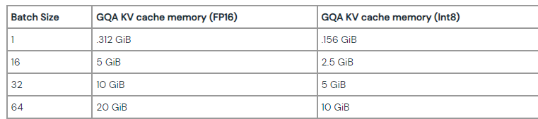
Table 3: KV cache size of LLaMA-2-70B when sequence length is 1024

Conclusion and Key Points

Each of the factors mentioned above affects how we build and deploy models. We use these results to make data-driven decisions, taking into account hardware type, software stack, model architecture, and typical usage patterns. Here are some suggestions based on our experience.

Clear optimization goals: Are you concerned about interactive performance? Is it to maximize throughput? Or do you want to minimize costs? There are predictable trade-offs.

Focus on the components of latency: For interactive applications, the time of the first word affects the response speed of your service, and the time of a single output word determines how good it feels. How fast.

Memory bandwidth is key: Generating the first token is often computationally limited, while subsequent decoding is memory limited. Since LLM inference typically runs in a memory-constrained environment, Memory Bandwidth Utilization (MBU) is a good metric to use to optimize and compare the efficiency of inference systems.

Batch processing is critical: The ability to process multiple requests simultaneously is critical to achieving high throughput and efficient utilization of expensive GPUs. Continuous batch processing is essential for shared online services, while offline batch inference workloads can achieve high throughput with simpler batch processing techniques.

Deep optimization: Standard inference optimization techniques (such as operator fusion, weight quantization) are very important for LLM, but it is equally important to explore deeper system optimizations, especially those that improve memory Utilize optimization techniques such as KV cache quantization.

Hardware configuration: Decisions on the hardware to be deployed should be based on the model type and expected workload. For example, when scaling to multiple GPUs, the MBU of a small model (such as MPT-7B) decreases faster than that of a larger model (such as LLaMA2-70B). Performance also tends to scale sub-linearly with higher degrees of tensor parallelism. Still, for smaller models, higher tensor parallelism may still make sense if traffic is higher or users are willing to pay a premium for lower latency.

Data-Driven Decisions: Understanding the theory is important, but we recommend always measuring end-to-end server performance. There are many reasons why inference deployment performance is lower than expected. The MBU may be unexpectedly reduced due to software inefficiency. Hardware differences between cloud service providers may also introduce unexpected conditions (we observed 8 There is a 2x latency difference between A100 servers).

Everyone else is watching

试用OneFlow: github.com/Oneflow-Inc/oneflow/http://github.com/Oneflow-Inc/oneflow/

Performance Engineering for Language Large Model Inference: Best Practices

Guess you like