[Chapter 5 (Convolution for the whole family!) Introduction to OpenCv convolution, image noise + blur, edge detection, morphological operations (popular understanding and contact with image convolution related operations!)]

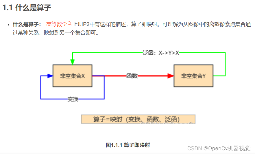
1 Introduction

1.1 Introduction to convolution

（1）卷积核：Whether it is the convolutional layer of CNN in the neural network , the filtering operation in OpenCv , or the morphological processing of binary images (multi-channel is also possible but not commonly used), convolution-related knowledge is used, and convolution is used. The kernel performs a sliding operation on the image. (Convolutions in neural networks are similar but not identical to convolutions in filtering ).

（2）CNN中的卷积：Convolution is commonly used in image processing, computer vision, speech recognition, natural language processing, text classification, pattern recognition, and other fields. In the image field , it can extract features from images and use them to better understand the content of the image. Convolution is usually used to detect edges , textures , objects and other features in images . It extracts features in the image by sliding a small filter (called a convolution kernel) and combines the extracted features to obtain better image analysis results.

（3）滤波中的卷积核：Image filtering is a technique for improving image quality by removing noise , blur , or other unwanted features from an image . It can also be used to increase the contrast of an image or to highlight edges or features in an image .

（4）形态学操作的卷积：After the image is preprocessed -> background and target segmentation, various noise points, holes, and slight connections often appear, so morphological operations are often used (similar to secondary processing of products). Among them, the convolution kernel ( structural element ) can be defined independently in morphological operations, and is divided into rectangle, cross, ellipse (a structural element definition method based on the drawing function will be shared in the morphological operation chapter later ); the main morphological operations Including corrosion, dilation, opening operation, closing operation, top hat, black hat, morphological gradient . Being familiar with the relevant theoretical knowledge of morphology will help us perform secondary processing of images, obtain the desired target contour, and select object frames.

（5）导语：Therefore, before learning deep learning, image blur, image edge extraction, and morphological operations, it is necessary to learn the basic knowledge of convolution.

1.2 Fuzzy operation

（1）作用：Blur operation is the most commonly used basic operation in image preprocessing, which can reduce noise , improve image quality, and reduce the complexity of subsequent algorithms.

（2）分类：Image blur is divided into mean, median, bilateral, Gaussian, and unsharp blur .

（3）导语：How to use these blur operations flexibly, so it is necessary to understand the underlying principles of various blurs and be able to select appropriate blur operations to preprocess the image according to different characteristics of the image.

1.3 Edge detection

（1）作用：Can be used to extract boundaries, contours, and textures.

（2）分类： The classification of image segmentation is mentioned in Chapter 3. Threshold segmentation belongs to the first category of background and target segmentation, and edge detection is the second category of segmentation. Edge detection can be divided into: based on differential operators, gradient operators, and Canny edge detection with the best effect.

（3）导语：Edge detection is also commonly used in cases such as lane line detection and perspective transformation in document correction. Therefore, it is necessary to understand edge detection algorithms and be able to flexibly choose background and target segmentation algorithms according to different scenarios.

1.4 Morphological operations

（1）作用：Morphological operations play a very important role in image processing. Its principle is based on the shape of the template (the shape of the convolution kernel). It can use corrosion, expansion, opening operations, closing operations, and other operations to extract image features. or for the purpose of segmenting the image.
（2）分类：Corrosion （缩小目标）, expansion （扩大目标）, opening operation （先腐蚀再膨胀）, closing operation (先膨胀再腐蚀), top hat operation （噪声=原图-开运算（先腐后膨））, black hat operation （空洞=闭运算（先膨后腐）-原图）, morphological gradient (物体边缘=原图-腐蚀), various mixed operations of expansion and erosion according to actual needs, etc.

（3）导语：When we segment the background and the target, there will be some holes, noise, or object connections. Therefore, it is necessary to perform morphological denoising, fill holes, or segment objects. It is therefore necessary to become familiar with morphological operations.

2. Introduction to convolution

2.1 Convolution operation

（1）卷积：

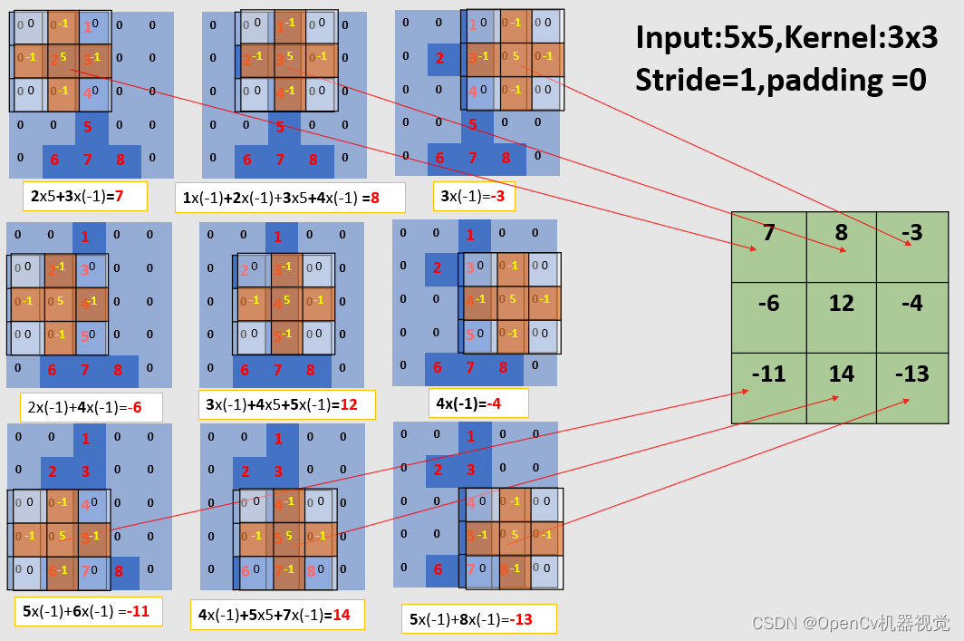
• The sliding convolution kernel window kernel slides on the input image Img, the overlapping areas are multiplied, and finally added, first horizontally , then vertically , and the output result is what we call a feature map. Because convolution is to extract features.

• Here Size(Img) is 5x5 and Size(Kernel) is 3x3. It can be seen from the figure that non-zero pixels form the number 1. Here, a convolution kernel commonly used for image sharpening is selected for demonstration.

• Convolution kernels are generally set to odd numbers such as: 1x1, 3x3, 5x5. Compared with even-numbered convolution kernels, a certain amount of calculation can be saved in convolution calculations; in filtering, the pairing of the filter can be ensured; at the same time, An odd number of convolution kernels makes it easier to find the center point and facilitate positioning. If there is an even number, positioning blur will occur.

  

Figure 2.1.1 Input image, convolution kernel

（2）卷积过程：

   As shown in the figure below, the convolution parameters are: stride is 1 and padding is 0. At this time, you can notice that the input image is 5x5 and the output feature map is 3x3 in size. When the number of convolutional layers of a deep learning network is very large, the feature map output after each convolution will be reduced , and will eventually be reduced to a size of 1x1. As a result, subsequent convolution calculations cannot be performed. Therefore a filling operation is required .

Figure 2.1.2 Convolution process

2.2 Filling (expanding the output feature map size)

（1）参数： 输入：5x5； 卷积核:3x3; 步幅:2; 填充：1（上下左右各填充1行/列）；输出：5x5。

(2)特点：According to the output feature map compared with the input feature map, the pixel value that makes up the number 1 is obviously larger , and the other pixel values ​​connected to it are obviously smaller , and the greater the difference between the two . This is the convolution kernel that selects the commonly used sharpening filter kernel , sum (convolution kernel) = 1 （>1则为亮度增强，<1降低亮度）, which you will see in the subsequent blur sharpening.

（3）注意点：While explaining the convolution operation, through this example, it is explained that the image is composed of pixel values. The larger the pixel value, the higher the brightness; the larger the difference between the outline pixel value and adjacent pixels, the stronger the contrast, which also belongs to image sharpening. ;

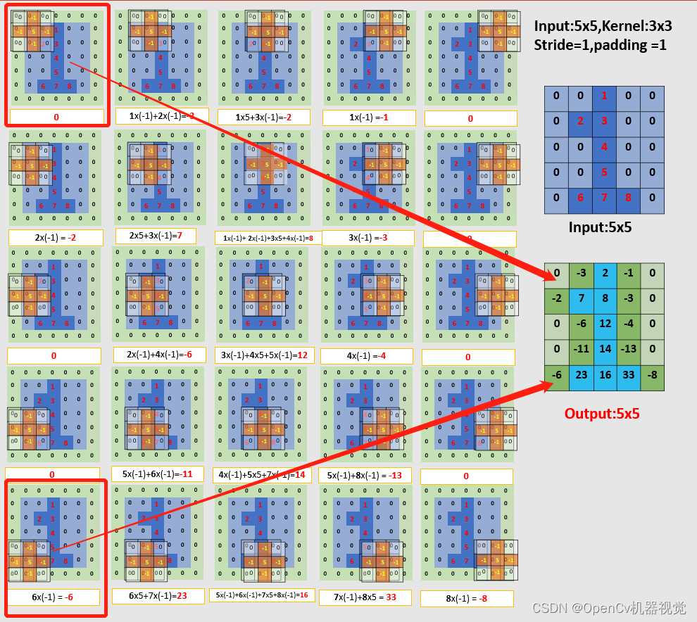
Figure 2.2.1 Convolution process (stride=1, padding=1)

• Because the overall screenshot range is wide, one screenshot per line below is for everyone’s convenience.

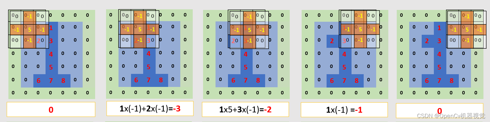
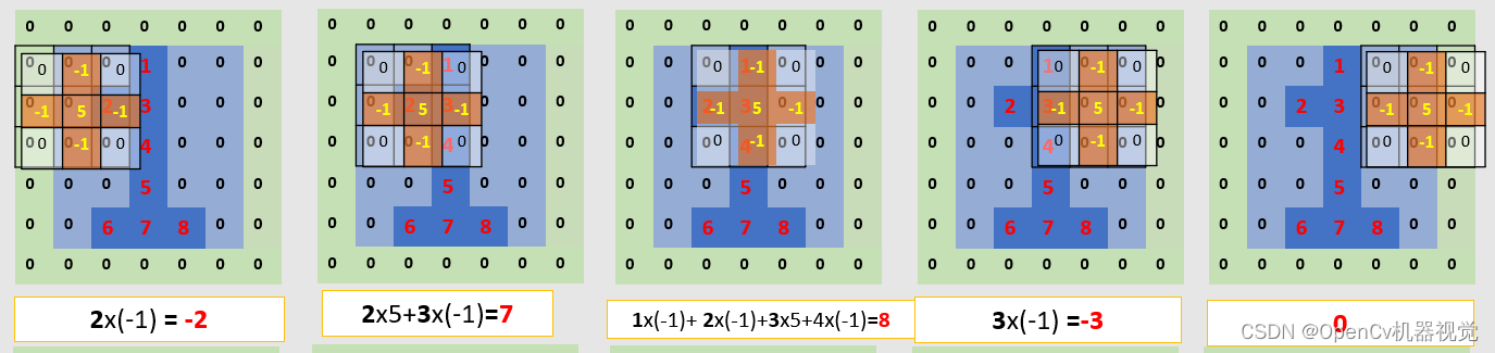
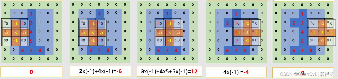
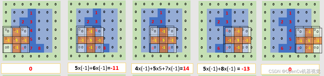
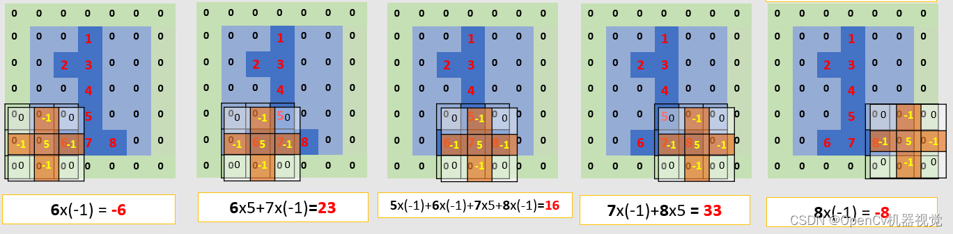
Figure 2.2.2 Convolution operation diagram

2.3 Stride (can reduce the size of the output feature map and reduce the amount of calculation for the next convolution)

（1）步幅：The convolution kernel moves at a pace. If the stride is not 1, assuming it is 2 ( 每次滑动两个单元）, the input feature map size of this example will become 3x3.

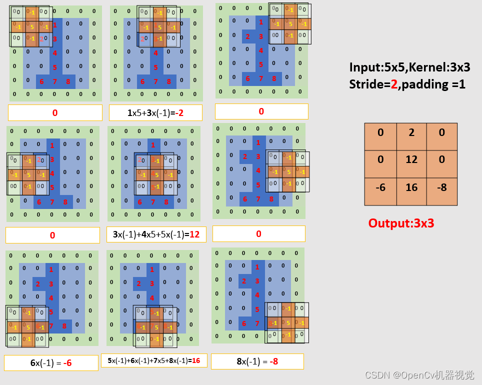
Figure 2.3.3 Convolution process (stride=2, padding=1)

（2）总结:When padding > 1, the size of the output feature map is increased to maintain the same size as the original image; when stride > 1, the size of the output feature map is reduced to reduce the amount of subsequent convolution calculations.

2.4 Calculation formula

*(1)备注： 输入大小（IH，IW);滤波器大小（FH.FW）;输出大小（OH,OW）;填充P，步幅S。
$$OH=\frac{IH+2P-FH}{S}+1(1)$$
$$OW=\frac{IW+2P-FW}{S}+1(2)$$

2.5 Verification code (implemented by Pytorch)

(1)代码：

import torch
import torch.nn.functional  as F
# 输入
input =torch.tensor([[0,0,1,0,0],
                    [0,2,3,0,0],
                    [0,0,4,0,0],
                    [0,0,5,0,0],
                    [0,6,7,8,0]])
# 卷积核
kernel = torch.tensor([[0,-1,0],
                      [-1,5,-1],
                      [0,-1,0]])

# nn卷积操作，数据格式是（batch_size,channel,h,w）
input = torch.reshape(input,(1,1,5,5))
kernel = torch.reshape(kernel,(1,1,3,3))
print(input)
print(kernel)

# 进行卷积操作,input:输入图像；kernel:卷积核；stride:步伐；,padding:填充，默认填充数据为0
output = F.conv2d(input,kernel,stride=2,padding=1)
print(output)

（2）卷积结果：Convolution is a mathematical operation and can be implemented in any language or python library we use. However, the most comprehensive implementation currently is the pytorch framework, which is the general trend.

tensor([[[[0, 0, 1, 0, 0],
          [0, 2, 3, 0, 0],
          [0, 0, 4, 0, 0],
          [0, 0, 5, 0, 0],
          [0, 6, 7, 8, 0]]]])
tensor([[[[ 0, -1,  0],
          [-1,  5, -1],
          [ 0, -1,  0]]]])
tensor([[[[ 0,  2,  0],
          [ 0, 12,  0],
          [-6, 16, -8]]]])

2.6 Recommended reading links

初衷：
1) Put recommended links. On the one hand, some of the content of this article refers to relevant links;
2) At the same time, I feel that these articles are quite well written and already have a very good wheel. There is no need to reinvent the same wheel;
3) Everyone based on To understand the level, choose to read, understand, and then synthesize based on multiple articles, so that you can have a thorough understanding of a point （个人觉得有很多文章，都有自己的定位以及亮点，很难单读一篇文章就全对该知识点理解得很透彻，但是看多了相关文章，学习每一篇文章的亮点之后，便会有自己的独特见解）.
4) It is convenient for everyone to find high-quality articles related to this knowledge point and improve efficiency.

1. Small mound, convolution explanation, easy to understand
2. The easiest to understand explanation of convolution
Note: The convolution in the signal processing system is basically the same as the convolution in OpenCV , but they still have some differences . Convolutions in signal processing systems are designed to manipulate signals, while OpenCV's convolutions are used for image processing. In addition, OpenCV's convolution operation provides more adjustable parameters, such as kernel size, stride, etc., while convolution in signal processing systems is simpler, with only one parameter, the shape of the signal. 3. Various
convolutions The most complete explanation of the accumulation method

2. Blurred image

导语：The blur operation mainly denoises the image . Therefore, before learning the blur operation, it is necessary to understand the types of noise . Combined with the characteristics of several blur processing, you can choose the appropriate blur algorithm according to the characteristics of the picture to blur the image. Improve image quality and reduce image processing complexity.

2.1 Introduction to common noise

2.1.1 Salt and pepper noise

（1）椒盐噪声：Salt and pepper spots in the image, which are maximum (white) or minimum (black) pixel values, their existence will affect the quality of the image;

（2）记忆方法:Black pepper ( black ), salt ( white ), when the image has black and white dots, median filtering can be used to remove noise. At the same time, you can simulate it by randomly adding bright and dark noise to the picture. Among them, the old black and white TV sets from the 1990s have snowflake screens that are actually salt and pepper noise. The color noise that appears on color televisions is Gaussian noise.

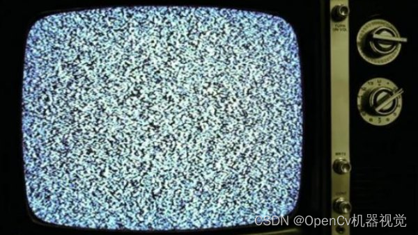
Figure 2.1.1.1 Snowflake screen (salt and pepper noise)

(3)代码:(Add salt and pepper noise to images)

# 作者：OpenCv机器视觉
# 时间：2023/1/21
# 功能：给图片添加椒盐噪声
import cv2 as cv
import numpy as np



# 添加椒盐噪声
def make_salt_pepper_noise(img):
    # 进行添加噪声
    for i in range(1000):
        # 椒（黑色）噪点,随机坐标
        xb = np.random.randint(0, w)
        yb = np.random.randint(0, h)
        # 盐（白色）噪点，随机坐标
        xw = np.random.randint(0, w)
        yw = np.random.randint(0, h)

        # 根据坐标进行添加早点
        img[yb, xb, :] = 255  # h,w,c,第一个参数是高度、第二个参数是宽度、第三个参数是通道数
        img[yw, xw, :] = 0  # h,w,c,第一个参数是高度、第二个参数是宽度、第三个参数是通道数

    return img

# 读取图片
img = cv.imread(".\\img\\lena.jpg")

# 获取图片,h,w,c参数
h,w,c=img.shape
# 添加椒盐噪声
img_msp = make_salt_pepper_noise(img.copy())
# 图像拼接
stack = np.hstack([img, img_msp])


# 显示图像
cv.namedWindow("img", 0)
cv.imshow("img", stack)
cv.waitKey(0)

(4)效果:It can be seen that the pixel difference of salt and pepper noise is large, the noise is more obvious, and the contrast between bright and dark points is strong, which makes it look more dazzling.

Figure 2.1.1.2 Original image (left), salt and pepper noise (right)

2.1.2 Random noise

（1）随机噪声：　Also known as background noise, it has no regularity and will affect the contrast and brightness of the image. Mean filtering has the best effect. 椒盐噪声，黑白点；高斯噪声彩色点，但是符合高斯分布;随机噪声个人理解，就是彩色噪声，同时不符合规律分布的就是随机噪声。(You can refer to article 1. My personal understanding is not comprehensive enough. Since random noise is very similar to salt and pepper noise, I will understand it in the way of salt and pepper noise. However, random noise does not have distribution rules. If you have a good understanding method, please comment in the comment area. Let’s discuss together.)

（2）代码：

# 作者：OpenCv机器视觉
# 时间：2023/1/24
# 功能：给图片添加随机噪声
import cv2 as cv
import numpy as np

# 生成随机噪声
def make_random_noise(img_noise, num=100):

    # 获取图片h,w,c参数
    h,w,c = img_noise.shape

    # 加噪声
    for i in range(num):
        b = np.random.randint(0,255)    # 每个通道数值随机生成
        g = np.random.randint(0,255)
        r = np.random.randint(0,255)

        x = np.random.randint(0, w)  # 随机生成指定范围的整数
        y = np.random.randint(0, h)
        img_noise[y, x] = (b,g,r)   # opencv读取图像后，是BGR格式

    return img_noise



img = cv.imread(".\\img\\lena.jpg")


# 生成随机噪声，噪声点数量没加，就按照函数默认参数100来
img_rn = make_random_noise(img.copy(),5000)
# 合并图像
stack = np.hstack([img,img_rn])

# 显示图像
cv.namedWindow("img", 0)
cv.imshow("img", stack)
cv.waitKey(0)

(3)效果：The noise distribution is irregular , color (color image)/black and white (grayscale image), a bit like the distribution of salt and pepper noise (black and white), because it is randomly generated; it is also a bit like Gaussian noise (color), but there is no distribution rule. You just need to know roughly what it is, and you don’t have to force it to remember it. It’s just irregular noise anyway.

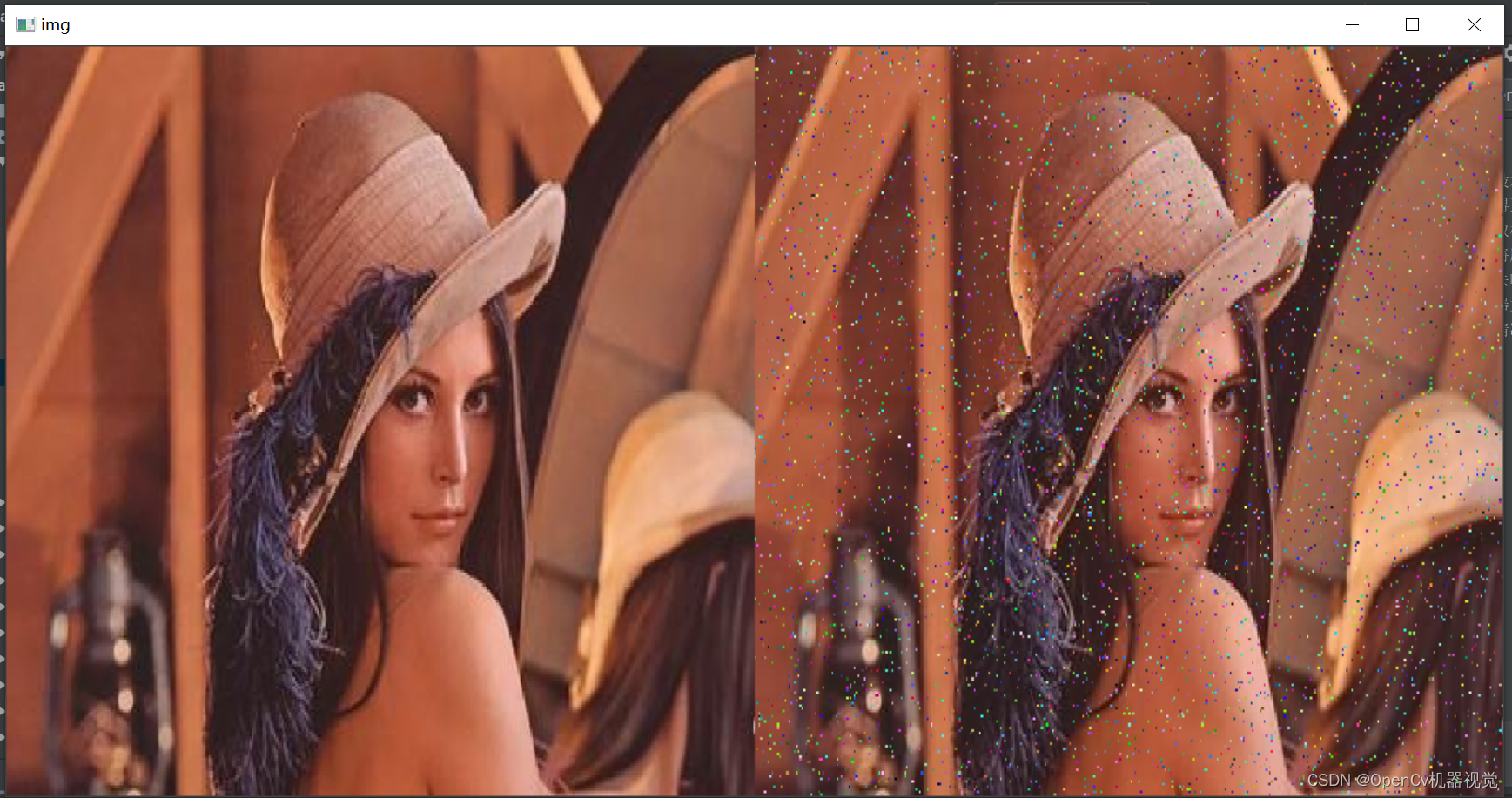
Figure 2.1.2.1 Original image (left) random noise (right)

2.1.3 Gaussian noise

(1)高斯噪声：Gaussian noise refers to random noise in an image, which degrades the quality of the image. Old-fashioned color TVs tend to have a lot of colored noise on rainy days , which is Gaussian noise (grayscale images also have Gaussian noise, but it is just gray noise).

Figure 2.1.3.1 Color TV noise (Gaussian noise)

(2)代码(Adding Gaussian noise to color images):

# 作者：OpenCv机器视觉
# 时间：2023/1/21
# 功能：给彩色图片添加高斯噪声

import numpy as np
import cv2 as cv



def make_gauss_noise(img, mean=0, sigma=25):
    img = np.array(img / 255, dtype=float)  # 将原始图像的像素值进行归一化,因为高斯分布是在0-1区间
    # 创建一个均值为mean，方差为sigma，呈高斯分布的图像矩阵
    noise = np.random.normal(mean, sigma / 255.0, img.shape)
    add = img + noise  # 将噪声和原始图像进行相加得到加噪后的图像
    img_mgn= np.clip(add, 0.0, 1.0)
    img_mgn = np.uint8(img_mgn * 255.0)

    return img_mgn

img = cv.imread(".\\img\\lena.jpg")
img_mgn = make_gauss_noise(img,0,np.random.randint(25,50))

# 图像拼接
stack = np.hstack([img, img_mgn])


# 显示图像
cv.namedWindow("img", 0)
cv.imshow("img", stack)
cv.waitKey(0)

(3)添加效果:

Figure 2.1.3.2 Original image (left), added Gaussian noise (right)

2.1.3 Recommended reading articles

1. Digital image processing: noise models (salt and pepper noise, random noise, Gaussian noise) and filtering methods
2. Image blur (mean, Gaussian, median, bilateral filtering)
3. Image motion blur
4. Image plus Gaussian noise

2.2 Motion blur

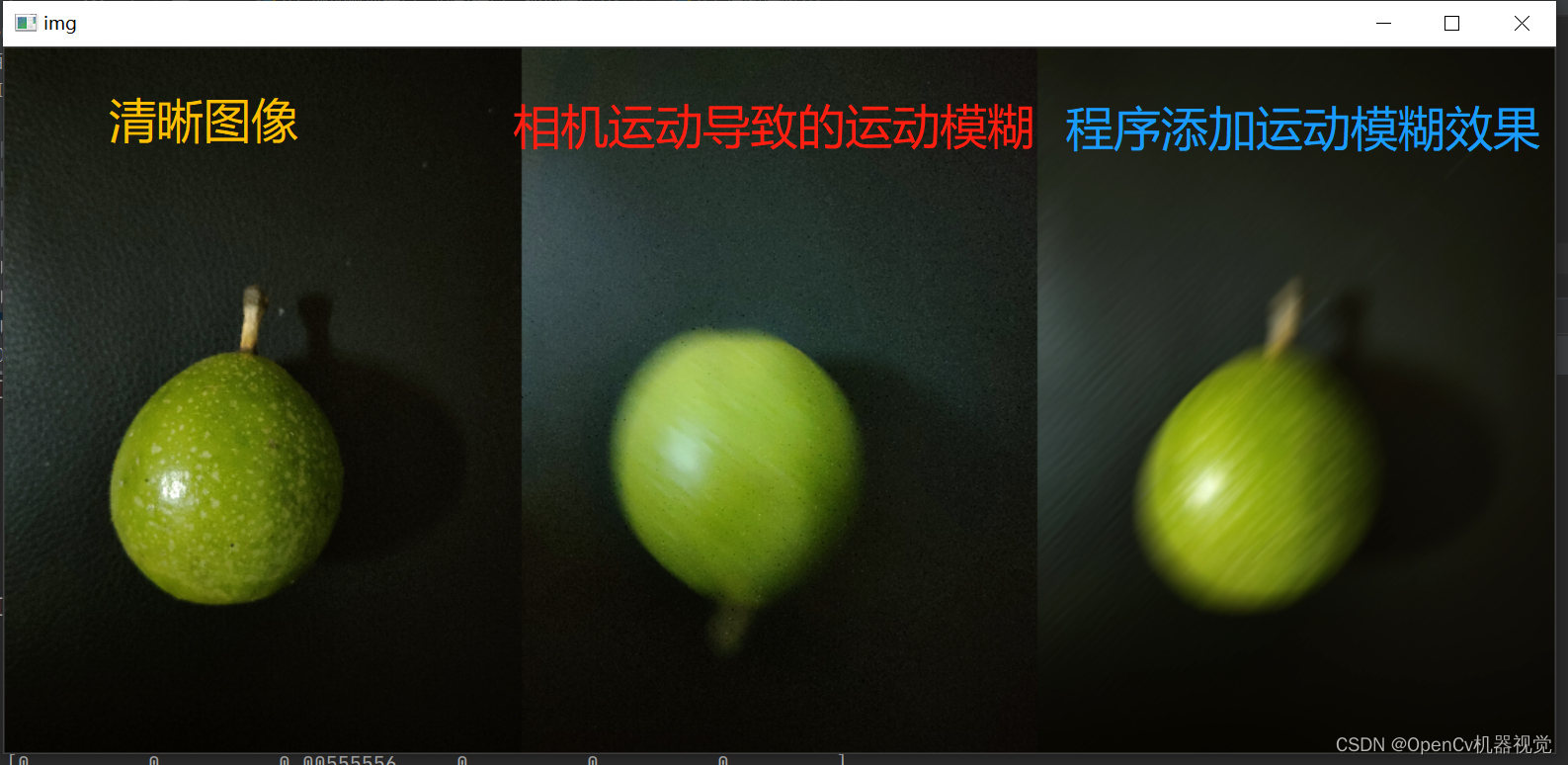
（1）运动模糊：It is caused by the relative movement speed of the camera or detection target being too fast (motion blur is often blurred in one direction ); therefore, when selecting a camera, we often need to consider the movement speed and frame rate of the object. If the movement speed is fast, , the frame rate is low, it is easy to cause motion blur. The solution to motion blur is to use a camera with a higher frame rate.

（2）代码：Add motion blur to images.

# 作者：OpenCv机器视觉
# 时间：2023/1/21
# 功能：给图片添加运动模糊效果
import cv2 as cv
import numpy as np

# 制作运动模糊
def make_motion_blur_noise(img, degree=180*1, angle=90):
    
    # 这里生成任意角度的运动模糊kernel的矩阵， degree越大，模糊程度越高
    M = cv.getRotationMatrix2D((degree/2, degree/2), angle, 1)
    print(M)

    motion_blur_kernel = np.diag(np.ones(degree))
    print(motion_blur_kernel)

    motion_blur_kernel = cv.warpAffine(motion_blur_kernel, M, (degree, degree))
    print(motion_blur_kernel)

    motion_blur_kernel = motion_blur_kernel / degree
    print(motion_blur_kernel)

    blurred = cv.filter2D(img, -1, motion_blur_kernel)
    
    # convert to uint8
    cv.normalize(blurred, blurred, 0, 255, cv.NORM_MINMAX)
    blurred = np.array(blurred, dtype=np.uint8)
    return blurred

# 清晰原图
img = cv.imread(".\\img\\bxg_clear.jpg")
# 由于相机移动导致的运动模糊
img_original_motion_blur = cv.imread(".\\img\\bxg_original_motion_blur.jpg")

# 制作运动模糊
img_motion_blur = make_motion_blur_noise(img)
# 图像水平拼接，np.vstack为垂直拼接
stack = np.hstack([img,img_original_motion_blur,img_motion_blur])


# 显示图像
cv.namedWindow("img",0)
cv.imshow("img",stack)
cv.waitKey(0)

（3）运动模糊效果：Left: clear original image; middle: motion blur caused by camera movement; right: using code to create a motion blur effect.

Figure 2.1.3 Motion blur comparison

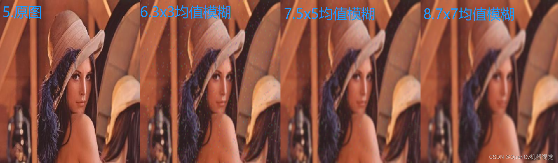
2. 3 Mean blur

(1)原理：The pixel values ​​around each pixel in the image (filter kernel coverage) are summed and averaged, and then this average is used to replace the original pixel value.

(2)类别：It is a linear (with a linear relationship, input and input are obtained by linear operations of pixel addition, subtraction , multiplication and division) filtering. Linear filtering also includes: median filtering, Gaussian filtering, and bilateral filtering. Common nonlinear filters include: dilation filtering and erosion filtering in morphological operations.
3）应用：Commonly used to remove random noise (application), because the calculation range is the range covered by the convolution kernel, so the larger the convolution kernel , the current pixel value is the mean value of the surrounding wider range of pixels, the greater the calculation amount , the denoising effect will be reduced The better , the more blurry and distorted the image will be, the more time-consuming it is to filter an image , and some details will be blurred. Because it is necessary to select the appropriate filter kernel size according to the actual situation.

（4）原理图解：Most of the filter kernels are odd numbers. Here, a matrix is ​​generated with 7x7size , and the mean filter kernel is 3x3.

• Mean fuzzy convolution kernel:
  $$Kernel=\frac{1}{K_w\ast K_h}\left(\begin{array}{ccccc}1& 1& \cdots & 1& \\ 1& 1& \cdots & 1& \\ ⋮& ⋮& \ddots & ⋮& \\ 1& 1& \cdots & 1& \end{array}\right)\text{\hspace{1em}(3)}$$

• The 3X3 convolution kernel is as follows:
  

Figure 2.3.1 3x3 mean filter kernel

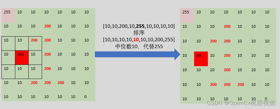
• Filtering process: Multiply & sum the filter kernel and the pixels covered by the image. Finally, assign this value to the dark red pixel. When the convolution kernel traverses and slides the entire image, the filtering is completed.

Figure 2.3.2 Filtering process

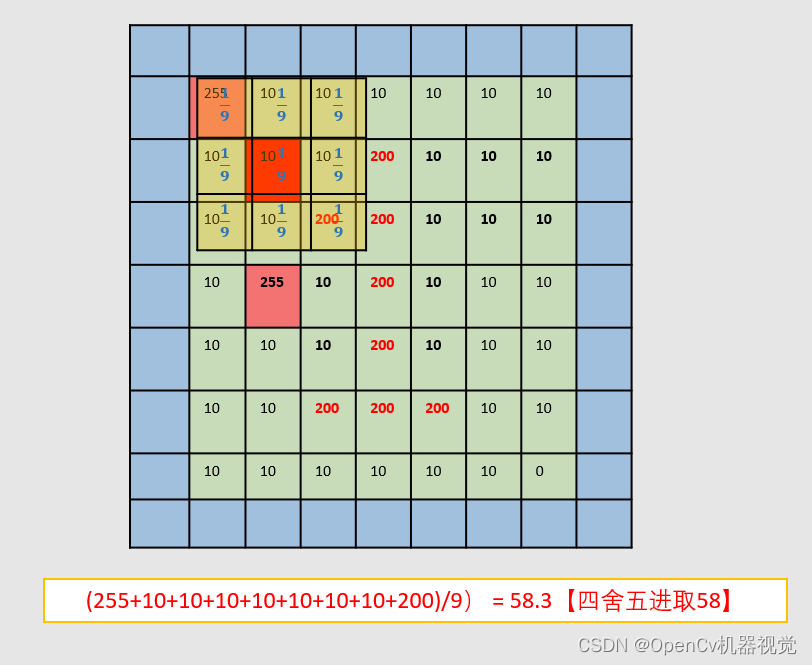
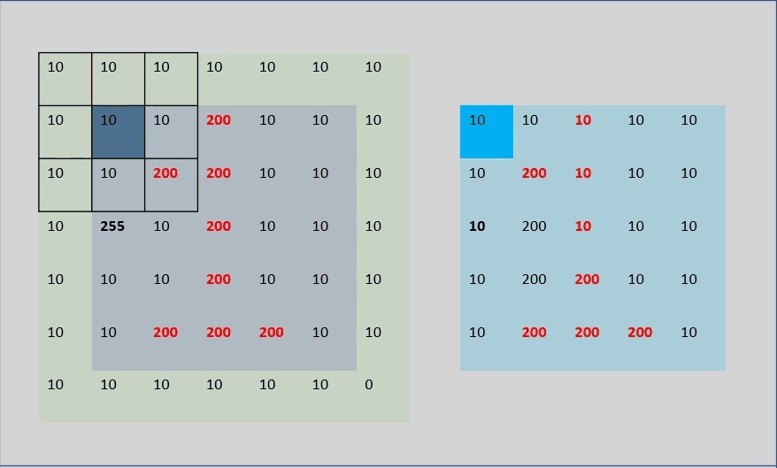
• Program operation result (the result is 58, marked with a mark)

均值滤波前:
[[255  10  10  10  10  10  10]
 [ 10  10  10 200  10  10  10]
 [ 10  10 200 200  10  10  10]
 [ 10 255  10 200  10  10  10]
 [ 10  10  10 200  10  10  10]
 [ 10  10 200 200 200  10  10]
 [ 10  10  10  10  10  10   0]]
均值滤波后:：
[[ 37  37  52  52  52  10  10]
 [ 37  《58》  73  73  52  10  10]
 [ 64  58 122  94  73  10  10]
 [ 64  58 122  94  73  10  10]
 [ 64  58 122 116  94  31  10]
 [ 10  31  73  94  73  30   9]
 [ 10  52  94 137  94  51   9]]

5.疑问？：Because the center pixel value of the filter kernel is the average pixel value of the filter kernel coverage, then the edge and four corner filter kernels will extend beyond the image. How is that calculated? (As shown below)

Figure 2.3.3 Boundary situation

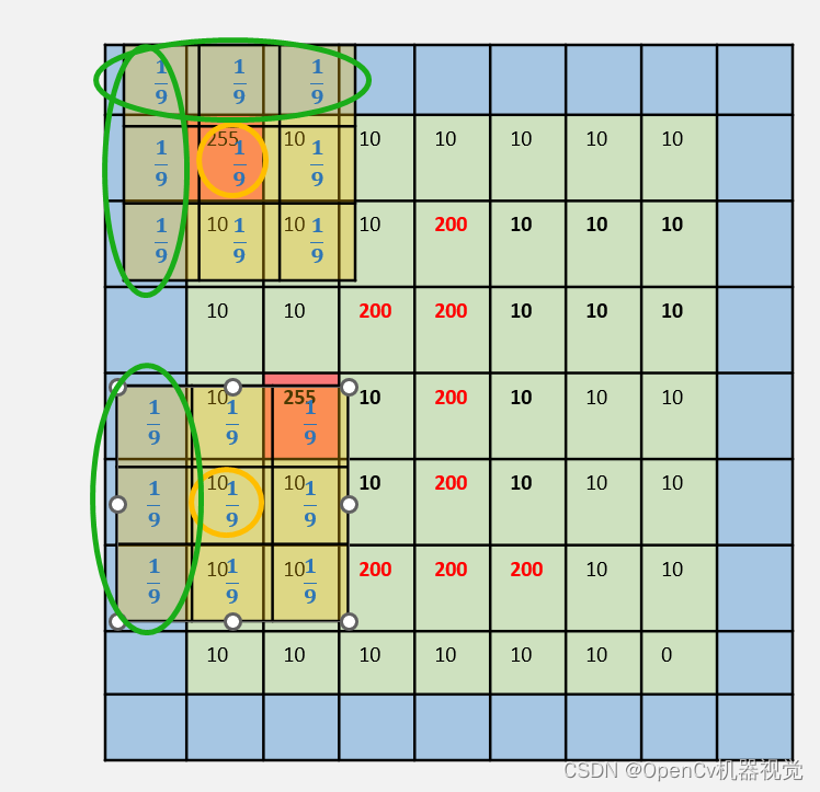
• Then raise a question: (1) If part of the filter kernel exceeds the image, then the filter kernel value is 1/9 or 1/(the number of pixels overlapping the filter kernel and the image) [verified by edges]; (2) The value of the upper left corner Does it have anything to do with the pixels in the attachment? (3) Do the relevant pixels contribute the same degree to the pixel value in the upper left corner? So I personally verified it through the code:

• After verification, (1): None; (2) (3) are related to the four pixels in the upper left corner. Each pixel has a different contribution, but it is symmetrical (img[0][1] and img[1][0 ] One of them changes the same value, and the img[0][0] value remains unchanged. img[1][1] changes the same value, but it changes). The pixels on the edge or four corners are actually in the form of expansion, but the filling value and calculation method are not clear (maybe due to limited personal understanding, or it may be related to the internal algorithm calculation method of opencv's API). Everyone Just directly understand the average value of surrounding pixels instead. If it is an edge, just fill it with 0 for auxiliary calculation. Comparing image edges is not our focus. I just had this question, so I found relevant articles to verify it, but basically it didn’t work. correct. (If you are interested, you can adjust the matrix value in the code for verification and testing. If there are good articles or four ways, you can discuss them in the comment area. We will update when we learn more later)

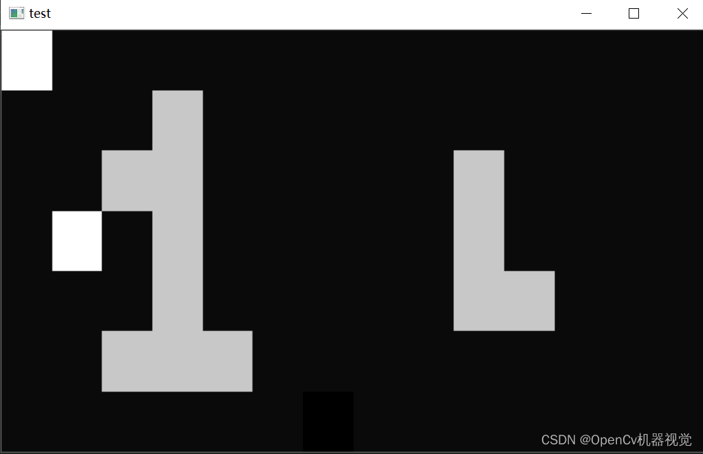
• Verification code: （大家可以修改矩阵值，进行验证） Here is to create a picture （方便打印查阅图像值）, blur it, and see the effect （也是进一步让大家了解图像其底层原理）.

# 作者：OpenCv机器视觉
# 时间：2023/1/22
# 功能：利用numpy创建图片（从像素解释模糊），添加椒盐噪声+均值模糊

import cv2 as cv
import numpy as np

# 创建图片
def test():

    # 创建一个全为0，大小为7x7的单通道矩阵
    img = np.array([[255,10,10,10,10,10,10],
                    [10,10,10,200,10,10,10],
                    [10,10,200,200,10,10,10],
                    [10,255,10,200,10,10,10],
                    [10,10,10,200,10,10,10],
                    [10,10,200,200,200,10,10],
                    [10,10,10,10,10,10,0]
                    ],dtype=np.uint8)
    print("均值滤波前:：")
    print(img)



    # 利用3x3的均值滤波核，对图像进行模糊
    blurred = cv.blur(img, (3, 3))
    print("均值滤波后:：")
    print(blurred)

    cv.namedWindow("test", 0)
    cv.imshow("test", np.hstack([img,blurred]))
	cv.waitKey(0)


img = cv.imread(".\\img\\lena.jpg")

# 获取图片,h,w,c参数
h,w,c=img.shape
test()

• Verification effect:
  The code simulates three salt and pepper noises (two white and one black). It can be seen that after mean filtering, the image is denoised, but it also becomes blurred. At the same time, the details of number 1 (the effect of removing salt and pepper noise is not so ideal).

Figure 2.3.4 Create pictures and average filtering effect

（6）随机噪声+椒盐噪声+高斯噪声对比 and 不同滤波核大小对图像的模糊降噪模糊效果 and 均值滤波对随机噪声、椒盐噪声、高斯噪声的去噪效果

• Code （部分代码会重复，主要是为了方便使用，直接全部复制，读取图片就可以看效果，不能自己过多操作）:

# 作者：OpenCv机器视觉
# 时间：2023/1/25
# 功能：随机噪声+椒盐噪声+高斯噪声对比 and 不同滤波核大小对图像的模糊降噪模糊效果 and 均值滤波对随机噪声、椒盐噪声、高斯噪声的去噪效果

import cv2 as cv
import numpy as np


# 添加高斯噪声
def make_gauss_noise(image, mean=0, sigma=25):
    image = np.array(image / 255, dtype=float)  # 将原始图像的像素值进行归一化,因为高斯分布是在0-1区间
    # 创建一个均值为mean，方差为sigma，呈高斯分布的图像矩阵
    noise = np.random.normal(mean, sigma / 255.0, image.shape)
    add = image + noise  # 将噪声和原始图像进行相加得到加噪后的图像
    img_noise= np.clip(add, 0.0, 1.0)
    img_noise = np.uint8(img_noise * 255.0)


    return img_noise
# 添加随机噪声
def make_random_noise(img_noise, num=100):

    # 获取图片h,w,c参数
    h,w,c = img_noise.shape

    # 加噪声
    for i in range(num):
        b = np.random.randint(0,255)    # 每个通道数值随机生成
        g = np.random.randint(0,255)
        r = np.random.randint(0,255)

        x = np.random.randint(0, w)  # 随机生成指定范围的整数
        y = np.random.randint(0, h)
        img_noise[y, x] = (b,g,r)   # opencv读取图像后，是BGR格式


    return img_noise
# 添加椒盐噪声
def make_salt_pepper_noise(img_noise):
    # 进行添加噪声
    for i in range(1000):
        # 椒（黑色）噪点,随机坐标
        xb = np.random.randint(0, w)
        yb = np.random.randint(0, h)
        # 盐（白色）噪点，随机坐标
        xw = np.random.randint(0, w)
        yw = np.random.randint(0, h)

        # 根据坐标进行添加早点
        img_noise[yb, xb, :] = 255  # h,w,c,第一个参数是高度、第二个参数是宽度、第三个参数是通道数
        img_noise[yw, xw, :] = 0  # h,w,c,第一个参数是高度、第二个参数是宽度、第三个参数是通道数

    return img_noise



# 读取图片
img = cv.imread(".\\img\\lena.jpg")

# 获取图片,h,w,c参数
h,w,c=img.shape

# 添加随机噪声、椒盐噪声、高斯噪声
img_rn= make_random_noise(img.copy(),2000)
img_spn = make_salt_pepper_noise(img.copy())
img_gn = make_gauss_noise(img.copy())
img_noise_stack = np.hstack([img,img_rn,img_spn,img_gn])


# 不同大小的滤波核的滤波效果
blurred_3 = cv.blur(img_rn, (3, 3))
blurred_5 = cv.blur(img_rn, (5, 5)) # 对本张图片，5x5的滤波效果较好
blurred_7 = cv.blur(img_rn, (7, 7))
img_diffsize_stack = np.hstack([img,blurred_3,blurred_5,blurred_7])

# 对高斯噪声图进行中值模糊
blurred_rn5  = cv.blur(img_rn,(5,5))
blurred_spn5 = cv.blur(img_spn, (5, 5))
blurred_gn5 = cv.blur(img_gn, (5, 5))
img_diffnoise_stack = np.hstack([img,blurred_rn5,blurred_spn5,blurred_gn5])



# 垂直拼凑图片
stack = np.vstack([img_noise_stack,img_diffsize_stack,img_diffnoise_stack])    #

# 显示图像
cv.namedWindow("img", 0)
cv.imshow("img", stack)
cv.waitKey(0)

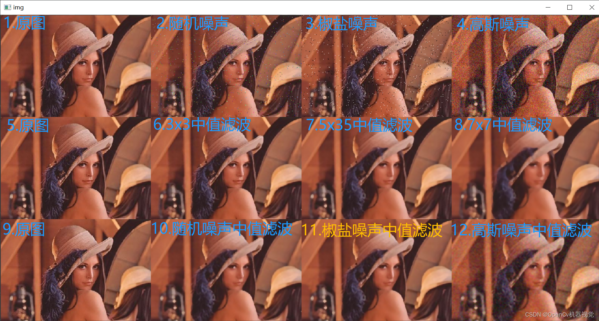
• Effect:

1）噪声对比: Figure 1-4, showing the original image, random noise, salt and pepper noise, and Gaussian noise images respectively.

2)滤波核大小影响：As can be seen from Figure 5-8, different convolution kernels have a better denoising effect on random noise, among which 5x5 has a better denoising effect. The larger the convolution kernel, the better the noise removal effect, the blurred image outline details, and the more distorted the image.

3）均值滤波对不同噪声的抑制效果：Figure 9-12 shows the comparison of the denoising effects of mean filter on different noises. It can be seen that mean filter has a relatively good suppression effect on random noise.
4）总结: The convolution kernel size is generally selected after weighing the pros and cons according to actual needs.

• renderings

Figure 2.3.5 Image blur effect

2.4 Median blur

(1)原理：Median filtering is a kind of nonlinear filtering . Its basic idea is to select a window on the image and replace the pixel value at the center point of the window with the median value of all pixel values ​​in the window . Because the median filter uses the median of the pixel values ​​in the window rather than the average of the pixel values, it can effectively suppress noise while retaining high spatial resolution.

（2）应用：Effectively remove salt and pepper noise.

（3）原理图解：

• After the filter kernel traverses the entire image, denoising is completed.

Figure 2.4.1. Median fuzzy principle

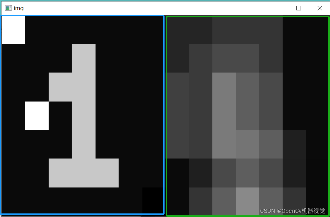
• Make a dynamic image to demonstrate median filtering. For the convenience of display, the size of the image is set to 5x5. GIF production tutorial reference [Chapter 2: OpenCv image, video reading and writing operations and basic applications]

Figure 2.4.2. Median fuzzy process

(4)创建图片，查看中值滤波后变换：Perform median blur on the created image (convenient for printing and checking image values)

• code

# 作者：OpenCv机器视觉
# 时间：2023/1/25
# 功能：创建一张图片进行中值滤波，并查看前后的像素值

import cv2 as cv
import numpy as np

# 函数说明，ctrl点cv.medianBlur就可以进入，里面有说明函数如何使用以及参数含义
"""
    medianBlur(src, ksize[, dst]) -> dst
    .   The function smoothes an image using the median filter 
    .   @param src input 1-, 3-, or 4-channel image; when ksize is 3 or 5, the image depth should be
    .   CV_8U, CV_16U, or CV_32F, for larger aperture sizes, it can only be CV_8U.
    .   @param dst destination array of the same size and type as src.
    .   @param ksize aperture linear size; it must be odd and greater than 1, for example: 3, 5, 7 ...

    """

# 创建图片进行中模糊
def test():

    # 创建一个全为0，大小为7x7的单通道矩阵
    img = np.array([[255,10,10,10,10,10,10],
                    [10,10,10,200,10,10,10],
                    [10,10,200,200,10,10,10],
                    [10,255,10,200,10,10,10],
                    [10,10,10,200,10,10,10],
                    [10,10,200,200,200,10,10],
                    [10,10,10,10,10,10,0]
                    ],dtype=np.uint8)
    print("中值滤波前:：")
    print(img)



    # 利用3x3的均值滤波核，对图像进行模糊
    blurred = cv.medianBlur(img, 3)
    print("中值滤波后:：")
    print(blurred)

    cv.namedWindow("test", 0)
    cv.imshow("test", np.hstack([img,blurred]))



test()
cv.waitKey(0)

• Output results: pixel values ​​before and after filtering: It can be seen that during median filtering of edge or diagonal pixel points, the filling is neither 0 nor 10. The specific expansion content is determined by the opencv median filtering algorithm, so it is the same as mean filtering. We won’t go into details here. The previous GIF was filled with 10. You can understand the process because edge information is not so important and important information is generally displayed in the center of the image.

均值滤波前:：
[[255  10  10  10  10  10  10]
 [ 10  10  10 200  10  10  10]
 [ 10  10 200 200  10  10  10]
 [ 10 255  10 200  10  10  10]
 [ 10  10  10 200  10  10  10]
 [ 10  10 200 200 200  10  10]
 [ 10  10  10  10  10  10   0]]
均值滤波后:：
[[ 10  10  10  10  10  10  10]
 [ 10  10  10  10  10  10  10]
 [ 10  10 200  10  10  10  10]
 [ 10  10 200  10  10  10  10]
 [ 10  10 200 200  10  10  10]
 [ 10  10  10  10  10  10  10]
 [ 10  10  10  10  10  10  10]]

• Filtering effect: It can better remove salt and pepper noise, while the overall brightness of the image remains unchanged, and the effect of removing salt and pepper noise is good.

Figure 2.4.3. Median blur results

（5)中值滤波对不同噪声的去除效果(The blur effect of mean filtering with convolution kernels of different sizes has been verified and will not be repeated later)

• code

# 作者：OpenCv机器视觉
# 时间：2023/1/25
# 功能：随机噪声+椒盐噪声+高斯噪声对比 and 不同滤波核大小对图像的模糊降噪模糊效果 and 中值滤波对随机噪声、椒盐噪声、高斯噪声的去噪效果


import cv2 as cv
import numpy as np

# 函数说明，ctrl点cv.medianBlur就可以进入，里面有说明函数如何使用以及参数含义
"""
    medianBlur(src, ksize[, dst]) -> dst
    .   The function smoothes an image using the median filter 
    .   @param src input 1-, 3-, or 4-channel image; when ksize is 3 or 5, the image depth should be
    .   CV_8U, CV_16U, or CV_32F, for larger aperture sizes, it can only be CV_8U.
    .   @param dst destination array of the same size and type as src.
    .   @param ksize aperture linear size; it must be odd and greater than 1, for example: 3, 5, 7 ...

    """

# 添加高斯噪声
def make_gauss_noise(image, mean=0, sigma=25):
    image = np.array(image / 255, dtype=float)  # 将原始图像的像素值进行归一化,因为高斯分布是在0-1区间
    # 创建一个均值为mean，方差为sigma，呈高斯分布的图像矩阵
    noise = np.random.normal(mean, sigma / 255.0, image.shape)
    add = image + noise  # 将噪声和原始图像进行相加得到加噪后的图像
    img_noise= np.clip(add, 0.0, 1.0)
    img_noise = np.uint8(img_noise * 255.0)


    return img_noise
# 添加随机噪声
def make_random_noise(img_noise, num=100):

    # 获取图片h,w,c参数
    h,w,c = img_noise.shape

    # 加噪声
    for i in range(num):
        b = np.random.randint(0,255)    # 每个通道数值随机生成
        g = np.random.randint(0,255)
        r = np.random.randint(0,255)

        x = np.random.randint(0, w)  # 随机生成指定范围的整数
        y = np.random.randint(0, h)
        img_noise[y, x] = (b,g,r)   # opencv读取图像后，是BGR格式


    return img_noise
# 添加椒盐噪声
def make_salt_pepper_noise(img_noise):
    # 进行添加噪声
    for i in range(1000):
        # 椒（黑色）噪点,随机坐标
        xb = np.random.randint(0, w)
        yb = np.random.randint(0, h)
        # 盐（白色）噪点，随机坐标
        xw = np.random.randint(0, w)
        yw = np.random.randint(0, h)

        # 根据坐标进行添加早点
        img_noise[yb, xb, :] = 255  # h,w,c,第一个参数是高度、第二个参数是宽度、第三个参数是通道数
        img_noise[yw, xw, :] = 0  # h,w,c,第一个参数是高度、第二个参数是宽度、第三个参数是通道数

    return img_noise



# 读取图片
img = cv.imread(".\\img\\lena.jpg")

# 获取图片,h,w,c参数
h,w,c=img.shape


# 添加随机噪声、椒盐噪声、高斯噪声
img_rn= make_random_noise(img.copy(),2000)
img_spn = make_salt_pepper_noise(img.copy())
img_gn = make_gauss_noise(img.copy())
img_noise_stack = np.hstack([img,img_rn,img_spn,img_gn])


# 不同大小的滤波核的滤波效果
blurred_3 = cv.medianBlur(img_spn, 3)
blurred_5 = cv.medianBlur(img_spn,5) # 对本张图片，5x5的滤波效果较好
blurred_7 = cv.medianBlur(img_spn, 7)
img_diffsize_stack = np.hstack([img,blurred_3,blurred_5,blurred_7])

# # 对随机噪声、椒盐噪声、高斯噪声噪声图进行中值模糊
blurred_rn5  = cv.medianBlur(img_rn,5)
blurred_spn5 = cv.medianBlur(img_spn, 5)
blurred_gn5 = cv.medianBlur(img_gn, 5)
img_diffnoise_stack = np.hstack([img,blurred_rn5,blurred_spn5,blurred_gn5])



# 垂直拼凑图片
stack = np.vstack([img_noise_stack,img_diffsize_stack,img_diffnoise_stack])    #

# 显示图像
cv.namedWindow("img", 0)
cv.imshow("img", stack)
cv.waitKey(0)

• Effect: Median filtering is very effective at removing salt and pepper noise （对高斯滤波的效果勉强还算可以，效果也跟高斯噪声参数设置有关，如噪声类型、质量）. The removal effect of different convolution kernel sizes is also very good, the brightness of the picture remains unchanged, and the original details of the picture are retained.

Figure 2.4.4. Comparison of the removal of different noises by median filtering

2.5 Gaussian blur

2.5.1 Gaussian blur

（1）原理：Different from mean filtering (replacing the pixel value of the center point of the window with all pixel values ​​in the window 均值) the weight of each pixel is the same, and the weights of the Gaussian distribution are based on the Gaussian distribution. The closer to the center point of the window, the greater the weight. The larger the value, the greater the impact on the center pixel.
（2）应用：Smooth images and eliminate Gaussian noise. :
（3）高斯分布概率密度分布函数: (具体原理见推荐阅读文章，里面讲得比较仔细，这里只是大致讲解一下）

• 一维：y=f(x)，$\mu$ (mean) determines the symmetry center,$\sigma$ (standard deviation),$p^2$ (variance) determines the shape of the distribution - the larger it is, the chunkier it is (the larger the variance, the greater the deviation from the mean, the wider the image, the area is 1, so the height is lower, so it is about chunky). In the same way, the more The smaller, the thinner and taller.

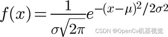
Figure 2.5.1.1 One-dimensional Gaussian distribution probability density formula

• One-dimensional normal distribution probability distribution image:

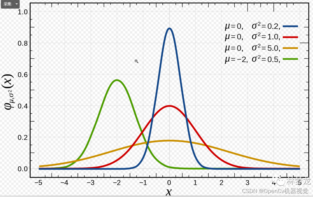
Figure 2.5.1.2 One-dimensional Gaussian distribution image

• Two dimensions: z = f(x,y),

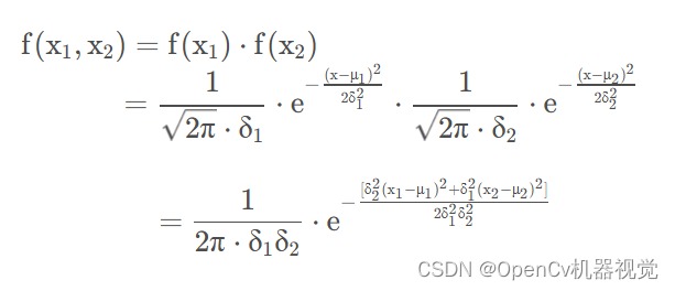
Figure 2.5.1.3 Two-dimensional Gaussian distribution probability density formula

• Two-dimensional Gaussian distribution:
  

Figure 2.5.1.4 Two-dimensional (image) Gaussian distribution image

• When the variance σ \sigma in each direction$When\; \sigma$ are all equal, the expression can be simplified as follows:
  

Figure 2.5.1.5 Two-dimensional (image) Gaussian distribution probability density formula

• The Gaussian kernel generated through Gaussian distribution is as follows: the closer to the center of the filter kernel, the greater the weight proportion, and the farther away, the smaller the weight proportion. From the X/Y dimension alone, it can be seen that it is very similar to the Gaussian distribution.

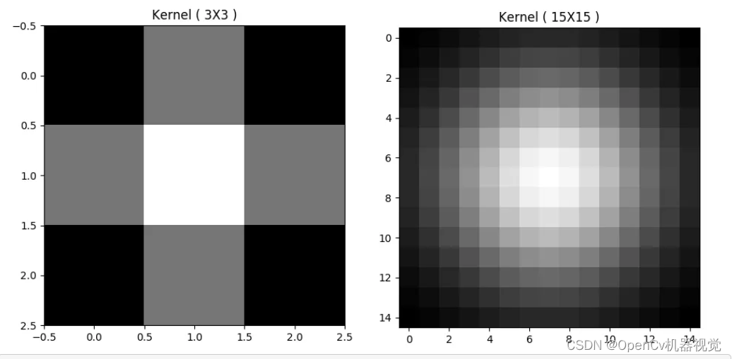
Figure 2.5.1.6 Two-dimensional (image) Gaussian distribution probability density formula

• Gaussian kernel generation code link: Refer to this link (reference link) and also add notes to everyone:

# 作者：OpenCv机器视觉
# 时间：2023/1/26
# 功能：生成高斯核
import cv2 as cv
import numpy as np
from matplotlib import pyplot as plt



def dnorm(x, mu, sd):
    """
    :param x:输入距离
    :param mu: 均值
    :param sd: 标准差
    """
    # 利用一维高斯分布函数进行计算
    return 1 / (np.sqrt(2 * np.pi) * sd) * np.e ** (-np.power((x - mu) / sd, 2) / 2)


def gaussian_kernel(size, sigma=1, verbose=False):
    # 高斯核其他像素点到中心点的距离，距离值之所以是这么计算，大家可以自行了解欧式距离等距离概念。
    kernel_1D = np.linspace(-(size // 2), size // 2, size)  # [-1.  0.  1.]

    # 根据距离，生成高斯分布的权重
    for i in range(size):                   #  [0.21296534 0.26596152 0.21296534]
        kernel_1D[i] = dnorm(kernel_1D[i], 0, sigma)


    # 滤波核是二维，且是实（数）对称矩阵，所以两个1维函数转置（对于1维结果还是1维，猜这里增加了转置可能是为了保证多维度计算的的对应）
    kernel_2D = np.outer(kernel_1D.T, kernel_1D.T)
    """
       Given two vectors, ``a = [a0, a1, ..., aM]`` and
    ``b = [b0, b1, ..., bN]``,
    the outer product [1]_ is::

      [[a0*b0  a0*b1 ... a0*bN ]
       [a1*b0    .
       [ ...          .
       [aM*b0            aM*bN ]]

    """

    # 进行归一化，卷积神经网络CNN中常对数据进行归一化，一方面是为了减少计算量，同时减少样本差异，归一化的方式也有多种，大家后续会学到
    kernel_2D *= 1.0 / kernel_2D.max()



    # 可以将像素以不同颜色进行显示，全总越大，颜色越深
    if verbose:
        plt.imshow(kernel_2D, interpolation='none', cmap='gray')   # 设置颜色
        plt.title("Image")
        plt.show()

    return kernel_2D

img_kernel = gaussian_kernel(3,1.5,1)
# 显示图像
cv.namedWindow("img", 0)
cv.imshow("img", img_kernel)
cv.waitKey(0)

（4）原理图解：(After thinking about it, I decided to perform a simulation operation)

• 1. Steps:
  1) Generate Gaussian convolution kernel: Gaussian distribution generates weights -> normalization
  2) Create pictures -> convolution

• 2. Similar to mean fuzzy, in filtering, the ideas are similar, and everyone should connect them in series to understand.

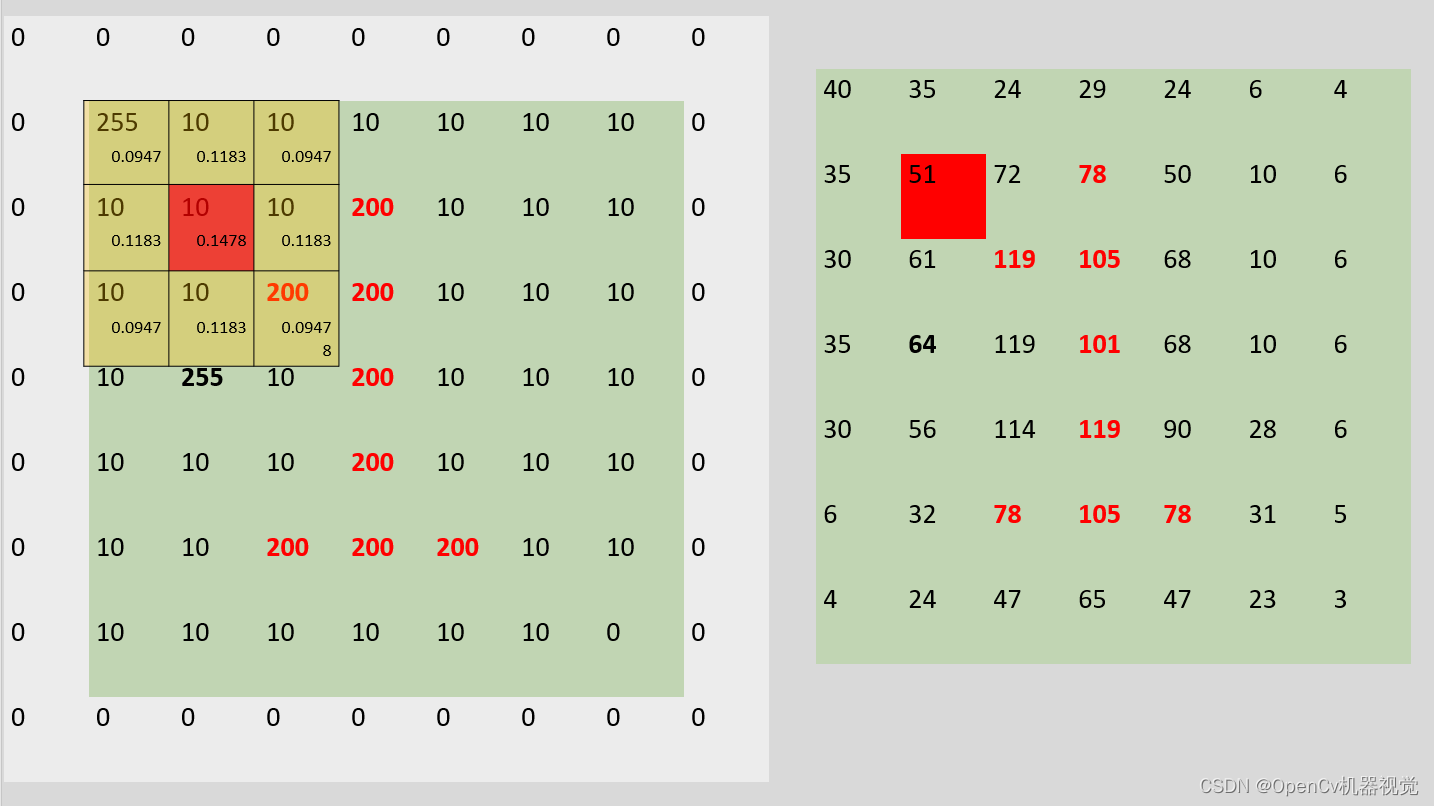
Figure 2.5.1.6 Gaussian filter principle

• 3. Principle verification code:(利用pytorch框架进行卷积运算，如果大家还没按照环境，可以根据第一章进行安装) :

# 作者：OpenCv机器视觉
# 时间：2023/1/26
# 功能：高斯原理演示

import cv2 as cv
import numpy as np
import torch
import torch.nn.functional  as F

# 高斯分布概率密度计算
def dnorm(x, mu, sd):
    """
    :param x:输入距离
    :param mu: 均值
    :param sd: 标准差
    """
    # 利用一维高斯分布函数进行计算
    return 1 / (np.sqrt(2 * np.pi) * sd) * np.e ** (-np.power((x - mu) / sd, 2) / 2)
# 获取高斯核
def gaussian_kernel(size, sigma=1, verbose=False):
    # 高斯核其他像素点到中心点的距离，距离值之所以是这么计算，大家可以自行了解欧式距离等距离概念。
    kernel_1D = np.linspace(-(size // 2), size // 2, size)  # [-1.  0.  1.]

    # 根据距离，生成高斯分布的权重
    for i in range(size):                   #  [0.21296534 0.26596152 0.21296534]
        kernel_1D[i] = dnorm(kernel_1D[i], 0, sigma)


    # 滤波核是二维，且是实（数）对称矩阵，所以两个1维函数转置（对于1维结果还是1维，猜这里增加了转置可能是为了保证多维度计算的的对应）
    kernel_2D = np.outer(kernel_1D.T, kernel_1D.T)
    """
       Given two vectors, ``a = [a0, a1, ..., aM]`` and
    ``b = [b0, b1, ..., bN]``,
    the outer product [1]_ is::

      [[a0*b0  a0*b1 ... a0*bN ]
       [a1*b0    .
       [ ...          .
       [aM*b0            aM*bN ]]

    """

    # 进行归一化，卷积神经网络CNN中常对数据进行归一化，一方面是为了减少计算量，同时减少样本差异，归一化的方式也有多种(除sum或者最大值，大家后续会学到
    # kernel_2D *= 1.0 / kernel_2D.max()    # x = x*x/max归一化
    print("归一化前:\n",kernel_2D)
    kernel_2D = kernel_2D / kernel_2D.sum()    # x = x*sum(x)归一化
    print("sum(kernel):" ,kernel_2D.sum())      # 归一化后，sum()=1,也就是图片总体亮度不变
    print("归一化后:\n",kernel_2D)


    return kernel_2D



# 获取高斯核
kernel = gaussian_kernel(3,1.5,1)


# 定义tensor二维数组，因为后面要卷积运算
input =torch.tensor([[255, 10, 10, 10, 10, 10, 10],
                    [10, 10, 10, 200, 10, 10, 10],
                    [10, 10, 200, 200, 10, 10, 10],
                    [10, 255, 10, 200, 10, 10, 10],
                    [10, 10, 10, 200, 10, 10, 10],
                    [10, 10, 200, 200, 200, 10, 10],
                    [10, 10, 10, 10, 10, 10, 0]
                    ],dtype=torch.float64)
# 转为图片，需要（h,w,c）格式，同时uint8
input_img = torch.reshape(input,(7,7))
input_img = np.array(input_img,np.uint8)


# 卷积前需要转为tensor格式
kernel = torch.tensor(kernel)   # np转tensor

# 转为卷积计算格式,batch_size,chancle,height,weight
input = torch.reshape(input,(1,1,7,7))
kernel = torch.reshape(kernel,(1,1,3,3))
print("input:\n",input)
print("kernel:\n",kernel)

# 卷积，为了保证输出大小不变，进行填充
output = F.conv2d(input,kernel,stride=1,padding=1)
output = torch.reshape(output,(7,7))    # 将维度转为7x7
output= np.array(output,np.uint8)      # 转为np格式，以及无符号Int类型，用于图片显示

blurred = cv.GaussianBlur(input_img, (3, 3), 0)
stack1 = np.hstack([input_img,output,blurred])
print("output:\n",output)
cv.namedWindow("img", 0)
cv.imshow("img", stack1)
cv.waitKey(0)

• 4. Running results:

归一化前:
 [[0.04535423 0.05664058 0.04535423]
 [0.05664058 0.07073553 0.05664058]
 [0.04535423 0.05664058 0.04535423]]
sum(kernel): 1.0000000000000002
归一化后:
 [[0.09474166 0.11831801 0.09474166]
 [0.11831801 0.14776132 0.11831801]
 [0.09474166 0.11831801 0.09474166]]
input:
 tensor([[[[255.,  10.,  10.,  10.,  10.,  10.,  10.],
          [ 10.,  10.,  10., 200.,  10.,  10.,  10.],
          [ 10.,  10., 200., 200.,  10.,  10.,  10.],
          [ 10., 255.,  10., 200.,  10.,  10.,  10.],
          [ 10.,  10.,  10., 200.,  10.,  10.,  10.],
          [ 10.,  10., 200., 200., 200.,  10.,  10.],
          [ 10.,  10.,  10.,  10.,  10.,  10.,   0.]]]], dtype=torch.float64)
kernel:
 tensor([[[[0.0947, 0.1183, 0.0947],
          [0.1183, 0.1478, 0.1183],
          [0.0947, 0.1183, 0.0947]]]], dtype=torch.float64)
output:
 [[ 40  35  24  29  24   6   4]
 [ 35  51  72  78  50  10   6]
 [ 30  61 119 105  68  10   6]
 [ 35  64 119 101  68  10   6]
 [ 30  56 114 119  90  28   6]
 [  6  32  78 105  78  31   5]
 [  4  24  47  65  47  23   3]]

• 5. Running effect: The blur effect is basically the same, but there is a slight difference from the Gaussian blur API of opencv. It may be caused by different variance parameter settings, or it may be due to different normalization functions, but the overall result is the same.

Figure 2.5.1.7 Gaussian simulation comparison

6. Effect analysis:　It can be seen intuitively that the pixel values ​​in the upper left corner and the last row are originally black pixels because there are brighter pixels around them. After Gaussian filtering, the pixel values ​​become higher. The overall contrast of the image signs decreases and becomes smoother and blurry.

Figure 2.5.1.8 Create pictures and apply Gaussian filtering effect

（4）高斯模糊实验代码：Several filtering codes are generally the same. What has changed is the filtering function. In order to copy first and use it first, it is better to paste them all.

# 作者：OpenCv机器视觉
# 时间：2023/1/25
# 功能：随机噪声+椒盐噪声+高斯噪声对比 and 不同滤波核大小对图像的模糊降噪模糊效果 and 高斯滤波对随机噪声、椒盐噪声、高斯噪声的去噪效果


import cv2 as cv
import numpy as np

# 函数说明，ctrl点cv.medianBlur就可以进入，里面有说明函数如何使用以及参数含义
"""
    GaussianBlur(src, ksize, sigmaX, dst=None, sigmaY=None, borderType=None)
    .   The function convolves the source image with the specified Gaussian kernel.
    .   @param src input image; the image can have any number of channels, which are processed
    .   independently, but the depth should be CV_8U, CV_16U, CV_16S, CV_32F or CV_64F.
    .   @param dst output image of the same size and type as src.
    .   @param ksize Gaussian kernel size. 
    .   @param sigmaX Gaussian kernel standard deviation in X direction.
    .   @param sigmaY Gaussian kernel standard deviation in Y direction; if sigmaY is zero, it is set to be
    .   equal to sigmaX, if both sigmas are zeros, they are computed from ksize.width and ksize.height,
    .   @param borderType pixel extrapolation method, see #BorderTypes.
    .   @sa  sepFilter2D, filter2D, blur, boxFilter, bilateralFilter, medianBlur
"""

# 添加高斯噪声
def make_gauss_noise(image, mean=0, sigma=15):
    image = np.array(image / 255, dtype=float)  # 将原始图像的像素值进行归一化,因为高斯分布是在0-1区间
    # 创建一个均值为mean，方差为sigma，呈高斯分布的图像矩阵
    noise = np.random.normal(mean, sigma / 255.0, image.shape)
    add = image + noise  # 将噪声和原始图像进行相加得到加噪后的图像
    img_noise= np.clip(add, 0.0, 1.0)
    img_noise = np.uint8(img_noise * 255.0)


    return img_noise
# 添加随机噪声
def make_random_noise(img_noise, num=100):

    # 获取图片h,w,c参数
    h,w,c = img_noise.shape

    # 加噪声
    for i in range(num):
        b = np.random.randint(0,255)    # 每个通道数值随机生成
        g = np.random.randint(0,255)
        r = np.random.randint(0,255)

        x = np.random.randint(0, w)  # 随机生成指定范围的整数
        y = np.random.randint(0, h)
        img_noise[y, x] = (b,g,r)   # opencv读取图像后，是BGR格式


    return img_noise
# 添加椒盐噪声
def make_salt_pepper_noise(img_noise):
    # 进行添加噪声
    for i in range(1000):
        # 椒（黑色）噪点,随机坐标
        xb = np.random.randint(0, w)
        yb = np.random.randint(0, h)
        # 盐（白色）噪点，随机坐标
        xw = np.random.randint(0, w)
        yw = np.random.randint(0, h)

        # 根据坐标进行添加早点
        img_noise[yb, xb, :] = 255  # h,w,c,第一个参数是高度、第二个参数是宽度、第三个参数是通道数
        img_noise[yw, xw, :] = 0  # h,w,c,第一个参数是高度、第二个参数是宽度、第三个参数是通道数

    return img_noise



# 读取图片
img = cv.imread(".\\img\\lena.jpg")
# 获取图片,h,w,c参数
h,w,c=img.shape



# 添加随机噪声、椒盐噪声、高斯噪声
img_rn= make_random_noise(img.copy(),2000)
img_spn = make_salt_pepper_noise(img.copy())
img_gn = make_gauss_noise(img.copy())
img_noise_stack = np.hstack([img,img_rn,img_spn,img_gn])


# 不同大小的滤波核的滤波效果
blurred_3 = cv.GaussianBlur(img_gn, (3,3),0)
blurred_5 = cv.GaussianBlur(img_gn,(5,5),0) # 对本张图片，5x5的滤波效果较好
blurred_7 = cv.GaussianBlur(img_gn, (7,7),0)
img_diffsize_stack = np.hstack([img,blurred_3,blurred_5,blurred_7])

# # 对随机噪声、椒盐噪声、高斯噪声噪声图进行高斯模糊
blurred_rn5  = cv.GaussianBlur(img_rn,(5,5),0)
blurred_spn5 = cv.GaussianBlur(img_spn, (5,5),0)
blurred_gn5 = cv.GaussianBlur(img_gn, (5,5),0)
img_diffnoise_stack = np.hstack([img,blurred_rn5,blurred_spn5,blurred_gn5])



# 垂直拼凑图片
stack = np.vstack([img_noise_stack,img_diffsize_stack,img_diffnoise_stack])    #

# 显示图像
cv.namedWindow("img", 0)
cv.imshow("img", stack)
cv.waitKey(0)

（5）效果：

• As can be seen from Figure 12, Gaussian filtering has a very good effect in removing Gaussian noise.

Figure 2.5.1.9 Comparison of the removal of different noises by Gaussian filtering

2.5.2 Stackblur blur (approximation of Gaussian blur)

（1）应用：For super-resolution images, if the convolution kernel is too large, the calculation will be very slow. Therefore, stackblur is an optimization algorithm proposed to address the slow operation of large convolution kernels. Stackblur algorithm introduction portal
（2）算法介绍：

2.6 Bilateral blurring

（1）原理：Bilateral filtering is an image processing technology that improves image quality. It can effectively retain image details while suppressing noise . It determines the pixel value based on the gray value of the image by calculating the Gaussian weighted distance between each pixel in the image and its neighbor pixels , thereby making the image edges clearer and noise more suppressed.简单来说，就是高斯模糊没有考虑到相邻像素的相似值，图像会总体比较模糊，双边滤波就是为了解决边缘模糊问题。

（2）应用：Compared with the previous blur operation, which blurs the edges of the contour, bilateral blur not only blurs the image but also preserves the edges of the contour well. It can be used for skin resurfacing , clear contours, and internal denoising.

（3）特点：Advantages: Reduces unwanted noise while maintaining edge contour details; Disadvantages: Slow calculation

（4）代码：

# 作者：OpenCv机器视觉
# 时间：2023/1/27
# 功能：随机噪声+椒盐噪声+高斯噪声对比 and 不同Sigma大小对图像的模糊降噪模糊效果 and 双边滤波对随机噪声、椒盐噪声、高斯噪声的去噪效果


import cv2 as cv
import numpy as np


# 函数说明，ctrl点cv.bilateralFilter就可以进入，里面有说明函数如何使用以及参数含义，

"""

    bilateralFilter(src, d, sigmaColor, sigmaSpace, dst=None, borderType=None)
     @brief Applies the bilateral filter to an image.
     
    .   The function 
    .   bilateralFilter can reduce unwanted noise very well while keeping edges fairly sharp. 
    .   However, it is very slow compared to most filters.
    .   
    .   src: 输入图像，可以是Mat类型，图像必须是8位或浮点型单通道、三通道的图像。 
    .  sigmaColor: 颜色空间过滤器的sigma值，这个参数的值越大，表明该像素邻域内有越宽广的颜色会被混合到一起，产生较大的半相等颜色区域。 
    .   sigmaSpace: 坐标空间中滤波器的sigma值，如果该值较大，则意味着越远的像素将相互影响，从而使更大的区域中足够相似的颜色获取相同的颜色。

    .   _Filter size_: Large filters (d \> 5) are very slow, so it is recommended to use d=5 for real-time
    .   applications, and perhaps d=9 for offline applications that need heavy noise filtering.
    
    .   _Sigma values_: For simplicity, you can set the 2 sigma values to be the same. If they are small (\<
    .   10), the filter will not have much effect, whereas if they are large (\> 150), they will have a very
    .   strong effect, making the image look "cartoonish".

"""


# 添加高斯噪声
def make_gauss_noise(image, mean=0, sigma=15):
    image = np.array(image / 255, dtype=float)  # 将原始图像的像素值进行归一化,因为高斯分布是在0-1区间
    # 创建一个均值为mean，方差为sigma，呈高斯分布的图像矩阵
    noise = np.random.normal(mean, sigma / 255.0, image.shape)
    add = image + noise  # 将噪声和原始图像进行相加得到加噪后的图像
    img_noise= np.clip(add, 0.0, 1.0)
    img_noise = np.uint8(img_noise * 255.0)


    return img_noise
# 添加随机噪声
def make_random_noise(img_noise, num=100):

    # 获取图片h,w,c参数
    h,w,c = img_noise.shape

    # 加噪声
    for i in range(num):
        b = np.random.randint(0,255)    # 每个通道数值随机生成
        g = np.random.randint(0,255)
        r = np.random.randint(0,255)

        x = np.random.randint(0, w)  # 随机生成指定范围的整数
        y = np.random.randint(0, h)
        img_noise[y, x] = (b,g,r)   # opencv读取图像后，是BGR格式


    return img_noise
# 添加椒盐噪声
def make_salt_pepper_noise(img_noise):
    # 进行添加噪声
    for i in range(1000):
        # 椒（黑色）噪点,随机坐标
        xb = np.random.randint(0, w)
        yb = np.random.randint(0, h)
        # 盐（白色）噪点，随机坐标
        xw = np.random.randint(0, w)
        yw = np.random.randint(0, h)

        # 根据坐标进行添加早点
        img_noise[yb, xb, :] = 255  # h,w,c,第一个参数是高度、第二个参数是宽度、第三个参数是通道数
        img_noise[yw, xw, :] = 0  # h,w,c,第一个参数是高度、第二个参数是宽度、第三个参数是通道数

    return img_noise



# 读取图片
img = cv.imread(".\\img\\lena.jpg")
# 获取图片,h,w,c参数
h,w,c=img.shape


# 添加随机噪声、椒盐噪声、高斯噪声
img_rn= make_random_noise(img.copy(),2000)
img_spn = make_salt_pepper_noise(img.copy())
img_gn = make_gauss_noise(img.copy())
img_noise_stack = np.hstack([img,img_rn,img_spn,img_gn])


# sigmaColor不同情况下的滤波效果
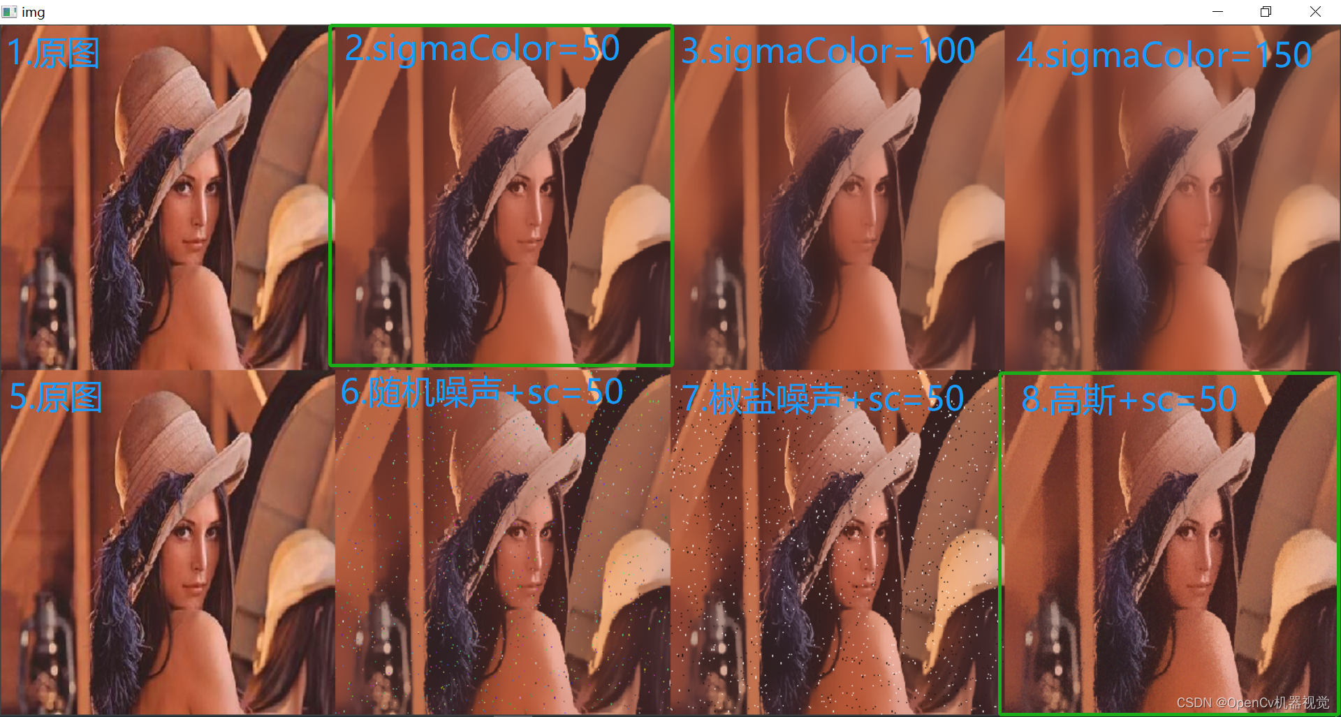
blurred_50 = cv.bilateralFilter(img, d=0, sigmaColor=50, sigmaSpace=15)# 双边保留滤波，经可能模糊其他背景，但是边缘保留下来。d 像素的领域直径，由颜色空间标准差sigmaColor（越大越好），坐标空间的标准差sigmaSpace（越小越好），决定
blurred_100 = cv.bilateralFilter(img, d=0, sigmaColor=100, sigmaSpace=15)
blurred_150 = cv.bilateralFilter(img, d=0, sigmaColor=150, sigmaSpace=15)
img_diffsize_stack = np.hstack([img,blurred_50,blurred_100,blurred_150])

# # 对随机噪声、椒盐噪声、高斯噪声噪声图进行双边滤波
blurred_rn5  = cv.bilateralFilter(img_rn, d=0, sigmaColor=50, sigmaSpace=15)
blurred_spn5 = cv.bilateralFilter(img_spn, d=0, sigmaColor=50, sigmaSpace=15)
blurred_gn5 = cv.bilateralFilter(img_gn, d=0, sigmaColor=50, sigmaSpace=15)
img_diffnoise_stack = np.hstack([img,blurred_rn5,blurred_spn5,blurred_gn5])



# 垂直拼凑图片
stack = np.vstack([img_diffsize_stack,img_diffnoise_stack])    #

# 显示图像
cv.namedWindow("img", 0)
cv.imshow("img", stack)
cv.waitKey(0)

（5）效果：The larger the sc parameter setting is, the wider the color range is considered and the blurr the image is; at the same time, it has a good suppression effect on Gaussian noise （具备高斯模糊分配权重的模糊特点，还具备保留边缘优点)while retaining the edges.

Figure 2.5.1.10 Bilateral filtering effect

（6） 推荐阅读文章：

1. Bilateral filter
1. Bilateral filter Popular understanding of bilateral filter
3. Bilateral filtering and code implementation

2.7 Summary

均值滤波：随机噪声
中值滤波：椒盐噪声
高斯滤波：高斯噪声
双边滤波：高斯噪声、在人物美艳磨皮中比较有效果。
自定义滤波：图像锐化、图像增强

2.8 Recommended reading articles

1. Analysis of the causes of motion blur/smear
2. Analysis in simple terms: cv2.getRotationMatrix2D

3. The principle of Gaussian blur
4. python+OpenCv notes (9): mean filtering
5. Median filtering (Median filtering)
6. Really understand mean blur, median blur, Gaussian blur, bilateral blur)
7. Gaussian blur)
8. Gaussian filtering)
9. Multidimensional Gaussian distribution
10. CV2 step-by-step learning-2: cv2.GaussianBlur() detailed explanation
11. OpenCv

Note: Knowledge related to the rotation matrix is ​​used in making motion blur cv.getRotationMatrix2D. This knowledge point is also commonly used in perspective transformation and rotation transformation in deep learning data enhancement . For now, you don’t have to worry about changing knowledge points. You can probably find out what motion blur looks like. After the basics are learned, I will learn cv.getRotationMatrix2Drelevant knowledge based on the project application. I will also update it and post a principle analysis article to prove it from the line generation. One article to solve the perspective transformation theory + practical application (will be updated later)

3. Edge detection

(1) Quote: The previous denoising is an important basic link in image preprocessing. In terms of edge detection, it mainly starts to segment the preprocessed image. Edge detection is widely used, and edge detection algorithms are often used in license plate inspection, road segmentation, and document correction.

Figure 3.1 Lane line detection
Figure 3.2 Document detection

(2) Implementation method: Edge detection is similar to CNN convolution, as well as the convolution of various blur filters. They are all convolution templates that operate on the image. It’s just that the templates are different. In edge detection, it can be divided into many operators. The following introduces its operator types and implementation effects one by one. (The concept of operators is mentioned in Chapter 3. )

Figure 3.3 Operator explanation

(3) This article first explains various edge detection operators one by one, and finally summarizes and compares the advantages and disadvantages of each operator. At the same time, many existing traditional algorithms in opencv are not very robust, and most of them need to be improved and applied (you can search for some algorithm improvement papers), but learning these algorithms is the basic premise. Only by understanding the basics can you stand on the shoulders of giants. Only by doing this can we write better algorithms.

3.1 Robert operator

（1）原理：An operator that uses local difference operators to find edges (局部区域内，相邻两个像素点值得变化，其导数可以用来衡量像素变化速度，如果变换较大，则大概率是边缘处). It can be divided into two templates, one in the x direction and one in the y direction.

（2）特点：The ability to suppress noise is weak. It detects horizontal and vertical lines better than arcs （与Sobel有些相反，见下面实验）. The edges are not very smooth, so the positioning is not very accurate.

（3）算子介绍：

Figure 3.1.1 Operator coordinates

• Gx operator

$$G_x=\left(\begin{array}{cc}1& 0\\ 0& -1\end{array}\right)\text{\hspace{1em}(4)}$$

• Gy operator
  $$G_x=\left(\begin{array}{cc}0& 1\\ -1& 0\end{array}\right)\text{\hspace{1em}(5)}$$

• G operator
  $$G=\sqrt{G_x^2+G_y^2}\text{\hspace{1em}(6)}$$

• Thesis explanation:

Figure 3.1.2 Gx, Gy, G paper description

（4）检测效果：

• 1.Original picture
  Figure 3.1.3 Original image of the experiment
  
  2. By the way, in order to observe the noise suppression effect of the Sobert operator, three different noises are added to the image: original image （左上）, random noise （右上）, salt and pepper noise （左下）, and Gaussian noise （右下）.
  Figure 3.1.4 Add noise map
  
• 3. Comparison before and after denoising: Robert算子抑制噪声较弱If the image has a lot of noise, the edge detection effect will be greatly reduced. Therefore, it needs to be denoised before edge detection.

Figure 3.1.4 Add noise map

• 4. $G_x$Operator detection, $G_x$Operator detection, $G_x$Comparison of operator detection: The lines in the diagonal direction formed by 0
     蓝色框： in the operator are well detected; at the same time, the oblique lines of 135° and 45° cannot be detected (you can refer to the principle code below to understand); x operator or y operator The arc detection lines are not continuous enough, but after weighting the two operators, the detection is still relatively complete; for some detections with relatively regular shapes (and without noise interference, if necessary, denoising is required), in fact, Robert calculates The edge detection effect is still good, but for some complex images, such as more diagonal lines and arcs, detection will be missed.
     绿色框：
黄色框：
总体来说：

Figure 3.1.5 Gx, Gy, G operator edge detection effect

• 5.Detection code:

"""
作者：OpenCv机器视觉
时间：2023/1/31
功能：1.利用roberts算子进行边缘检测，看GX、Gy、G算子检测不同角度直线+圆弧下的效果;
    2.添加噪声以及除噪后的实验对比

"""
import cv2 as cv
import numpy as np


# 添加高斯噪声
def make_gauss_noise(image, mean=0, sigma=15):
    image = np.array(image / 255, dtype=float)  # 将原始图像的像素值进行归一化,因为高斯分布是在0-1区间
    # 创建一个均值为mean，方差为sigma，呈高斯分布的图像矩阵
    noise = np.random.normal(mean, sigma / 255.0, image.shape)
    add = image + noise  # 将噪声和原始图像进行相加得到加噪后的图像
    img_noise= np.clip(add, 0.0, 1.0)
    img_noise = np.uint8(img_noise * 255.0)


    return img_noise
# 添加随机噪声
def make_random_noise(img_noise, num=300):

    # 获取图片h,w,c参数
    h,w,c = img_noise.shape

    # 加噪声
    for i in range(num):
        b = np.random.randint(0,255)    # 每个通道数值随机生成
        g = np.random.randint(0,255)
        r = np.random.randint(0,255)

        x = np.random.randint(0, w)  # 随机生成指定范围的整数
        y = np.random.randint(0, h)
        img_noise[y, x] = (b,g,r)   # opencv读取图像后，是BGR格式


    return img_noise
# 添加椒盐噪声
def make_salt_pepper_noise(img_noise):
    h,w = img_noise.shape[:2]
    print(h,w)
    # 进行添加噪声
    for i in range(500):
        # 椒（黑色）噪点,随机坐标
        xb = np.random.randint(0, w)
        yb = np.random.randint(0, h)
        # 盐（白色）噪点，随机坐标
        xw = np.random.randint(0, w)
        yw = np.random.randint(0, h)

        # 根据坐标进行添加早点
        img_noise[yb, xb, :] = 255  # h,w,c,第一个参数是高度、第二个参数是宽度、第三个参数是通道数
        img_noise[yw, xw, :] = 0  # h,w,c,第一个参数是高度、第二个参数是宽度、第三个参数是通道数

    return img_noise









# 左上角原图、右上角随机噪声、左下角椒盐噪声、右下角高斯噪声
img= cv.imread(".\\img\\1.jpg")
h,w,c = img.shape
mh,mw = h//2,w//2
img_top_r = img[0:mh,mw:w:]
img_under_l=img[mh:h,0:mw,:]
img_under_r = img[mh:h,mw:w:,:]
#　加噪声
# img_top_r = make_random_noise(img_top_r)
# img_under_l = make_salt_pepper_noise(img_under_l)
# img_under_r = make_gauss_noise(img_under_r)
# # 去噪
# img_top_r = cv.blur(img_top_r, (5, 5))
# img_under_l=cv.medianBlur(img_under_l, 3)
# img_under_r = cv.GaussianBlur(img_under_r,(5,5),0)

img[0:mh,mw:w:] = img_top_r
img[mh:h,0:mw,:] = img_under_l
img[mh:h,mw:w:,:] = img_under_r



gray= cv.cvtColor(img,cv.COLOR_BGR2GRAY)        #　转灰度
ret,binary = cv.threshold(gray,10,255,cv.THRESH_BINARY)   # 二值化

# robert算子定义
kernel_x = np.array([[1,0],[0,-1]],np.int8)
kernel_y = np.array([[0,1],[-1,0]],np.int8)

# robert算子检测
x=cv.filter2D(binary,cv.CV_16S,kernel_x)     # 可以看成卷积运算，原理通卷积但是又有些区别
y=cv.filter2D(binary,cv.CV_16S,kernel_y)    
absX = cv.convertScaleAbs(x)                # 因为算子中有-1，所以卷积后有部分是负数，需要取绝对值
absY = cv.convertScaleAbs(y)
Roberts = cv.addWeighted(absX,0.5,absY,0.5,0)   #  GX、Gy合成G
print(x[199])
print(absX[199])


stack = np.hstack([absX,absY,Roberts])

# 显示图片
cv.namedWindow("img",0)
cv.imshow("img",img)
cv.namedWindow("stack",0)
cv.imshow("stack",stack)
cv.namedWindow("Gx",0)
cv.imshow("Gx",absX)
cv.namedWindow("Gy",0)
cv.imshow("Gy",absY)
cv.namedWindow("G",0)
cv.imshow("G",Roberts)
cv.waitKey(0)

(5)边缘检测算子卷积原理演示：

• 1. In fact, to put it bluntly, it is the principle of convolution, but the operator (the same as the convolution kernel and the filter kernel, the names are different in different applications) is called an Robertoperator.

Figure 3.1.6 Code implementation effect

• 2. Simulation effect:
     Figure 3.1.6 Code implementation effect
     
• 3. Implementation code:

"""
作者：OpenCv机器视觉
时间：2023/1/31
功能：模拟Robert原理

"""

import cv2 as cv
import numpy as np


# 底层原理，输出结果与cv.fliter2D的结果会发生做偏移1个像素
def robert_x_y(img,kernel):
    # 复制一张原图
    result = img.copy()

    # 对图像进行扩充1行1列，用于边缘的计算
    h, w = img.shape
    add_r = np.zeros((1,w))
    add_c = np.zeros((h+1,1))    # 后增加的需要多加多一个角点
    img = np.row_stack((img,add_r))
    img = np.column_stack((img,add_c))
    h, w = img.shape

     # 平滑图像进行卷积运算
    for i in range(h):
        for j in range(w):
            if (i+2 < h) and (j+2 < w):
                roi = img[i:i + 2, j:j + 2]
                list_robert = kernel * roi
                result[i, j] = abs(list_robert.sum())  # 求和加绝对值
                print('{' ':>9}'.format(abs(list_robert.sum())),end='') # 输出右对齐
        print()
    return  result




input = np.array([[0, 0, 0, 0, 0, 0, 0],
                    [0, 0, 0, 0, 0, 0, 0],
                    [0, 0, 255, 255, 255, 0, 0],
                    [0, 0, 255, 255, 255, 0, 0],
                    [0, 0, 255, 255, 255, 0, 0],
                    [0, 0, 0, 0, 0, 0, 0],
                    [0, 0, 0, 0, 0, 0, 0]
                    ],dtype=np.uint8)





# robert算子定义
kernel_x = np.array([[1,0],[0,-1]],np.int8)
kernel_y = np.array([[0,1],[-1,0]],np.int8)

# 自己实现的函数
robertx= robert_x_y(input,kernel_x)
roberty= robert_x_y(input,kernel_y)
robertxy = cv.addWeighted(robertx,0.5,roberty,0.5,0)

#调用Opencv的函数
x=cv.filter2D(input,cv.CV_16S,kernel_x)
y=cv.filter2D(input,cv.CV_16S,kernel_y)
absX = cv.convertScaleAbs(x)
absY = cv.convertScaleAbs(y)
Roberts = cv.addWeighted(absX,0.5,absY,0.5,0)

# 图片拼接
stack1 = np.hstack([robertx,roberty,robertxy])
stack2 = np.hstack([absX,absY,Roberts])
stack = np.vstack([stack1,stack2])


cv.namedWindow("input",0)
cv.imshow("input",input)

cv.namedWindow("stack",0)
cv.imshow("stack",stack)

cv.waitKey(0)

(6)推荐阅读文章：

1. Robert operator for image segmentation
2. Robert operator for edge detection
Link: link

3.2 Sobel operator

（1）原理：Detect edges based on the gradient information of the image.
（2）特点：It is short in time, has certain noise immunity, and has good edge detection effect.

（3）算子介绍：

• 1. Similar to Robert , but the operator template is different. It is divided into horizontal template (can be understood as convolution kernel) and vertical template （两个互为转置，A[i][j]=B[j][i]）.

Figure 3.1.6 Code implementation effect

（4）检测效果：
1. Test the original image: Same as above.
2. In order to measure the anti-noise ability of the Sobel operator, add three types of noise to the image, same as above.
3. Comparison before and after denoising: Sobel operator has certain noise immunity.

(5)边缘检测算子卷积原理演示：
(6)推荐阅读文章：
[200 OpenCV routines] 64. Image sharpening - Sobel operator
https://blog.csdn.net/youcans/article/details/122152278
python+OpenCV image processing (8) Edge detection
https://blog. csdn.net/qq_40962368/article/details/81416954
OpenCV——Sobel edge detection
https://blog.csdn.net/qq_36686437/article/details/120814041
Sobel edge detection
https://www.cnblogs.com/yibeimingyue/p /10878514.html

3.3Scharra operator

（1）原理：
（2）特点：
（3）算子介绍：
（4）检测效果：
(5)边缘检测算子卷积原理演示：
(6)推荐阅读文章：

3.4 Prewitt operator

（1）原理：
（2）特点：
（3）算子介绍：
（4）检测效果：
(5)边缘检测算子卷积原理演示：
(6)推荐阅读文章：

3.5 Kirsh operator

（1）原理：
（2）特点：
（3）算子介绍：
（4）检测效果：
(5)边缘检测算子卷积原理演示：
(6)推荐阅读文章：

3.6 Robinson operator

（1）原理：
（2）特点：
（3）算子介绍：
（4）检测效果：
(5)边缘检测算子卷积原理演示：
(6)推荐阅读文章：

3.7 Laplacian operator

（1）原理：
（2）特点：
（3）算子介绍：
（4）检测效果：
(5)边缘检测算子卷积原理演示：
(6)推荐阅读文章：

3.8 Canny operator

（1）原理：
（2）特点：
（3）算子介绍：
（4）检测效果：
(5)边缘检测算子卷积原理演示：
(6)推荐阅读文章：

3.9 Edge detection with deep learning

(1) Advantages:
(2) Recommended model:
Comparison of various differential operators for edge detection (Sobel, Robert, Prewitt, Laplacian, Canny)
https://www.cnblogs.com/molakejin/p/5683372.html

Comparison of edge detection codes + effects of different operators

Recommended reading articles

• In edge detection, knowing its application, what methods are there to achieve edge detection? What is the effect of each edge detection method? Which edge detection algorithm is better. Then for the specific principles, you can refer to the following article. I will put some well-written articles here for everyone to read.

Recommended reading articles

1. Digital image processing: Edge detection (Edge detection)
Python image sharpening and edge detection (Roberts, Prewitt, Sobel, Lapllacian, Canny, LOG) >
Real product case: Implementing document edge detection
traditional edge detection operator
straight line detection algorithm Summarize several missing source codes in the straight line detection algorithm blog post (Hough_line, LSD, FLD, EDlines, LSWMS, CannyLines, MCMLSD, LSM)

4. Morphological operations

4.1 Corrosion

4.2 Expansion

4.3 Open operation

4.4 Closing operation

4.5 top hat

4.6 Black Hat:

4.7 Morphological gradient: