Hello everyone, today I will summarize for you the python machine learning fusion model: Stacking and Blending (with code).
1 Stacking method Stacking
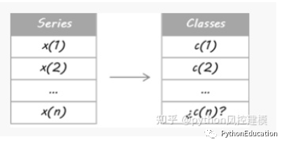
Can a weak system become a strong system?
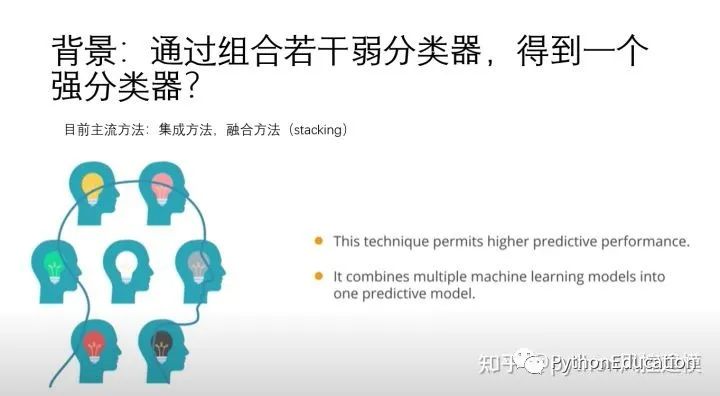
When you are faced with a complex classification problem, as is often the case in financial markets, different approaches may emerge when searching for a solution . Although these methods can estimate classifications, sometimes none of them is better than other classifications. In this case, the logical choice is to keep them all and then create the final system by integrating the parts. This diversified approach is one of the most convenient: split your decision between several systems to avoid putting all your eggs in one basket.
Once I have a large number of estimates for this situation, how can I combine the decisions of N subsystems? As a quick answer, I can make an average decision and use it. But is there a different way to fully utilize my subsystem? Of course!
Think creatively!
Several classifiers with a common goal are called multi-classifiers . In machine learning, a multi-classifier is a set of different classifiers that are estimated and fused together to get a result that combines them. Many terms are used to refer to multi-classifiers: multi-model, multi-classifier system, combination classifier, decision committee, etc. They can be divided into two main categories:
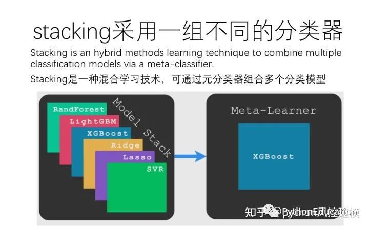
Integrated approach: refers to using the same learning technology to combine a set of systems to create a new system. Bagging and lifting are the most extended. Hybrid methods: taking a diverse group of learners and combining them using new learning technologies. Stacking (or stacked generalization) is one of the main hybrid multi-classifiers.
How to build a multi-classifier powered by Stacking.
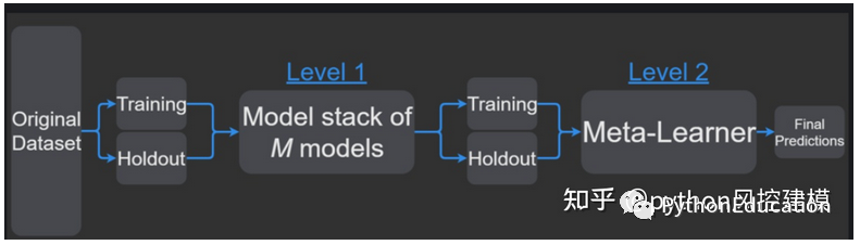
stacking workflow

.
Meta-classifiers can be trained on predicted class labels or on predicted class probabilities.
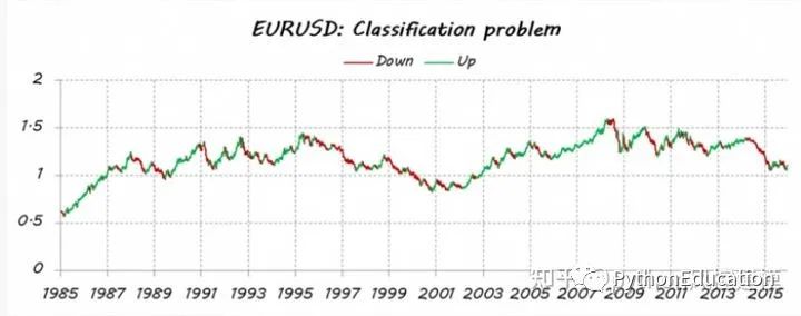
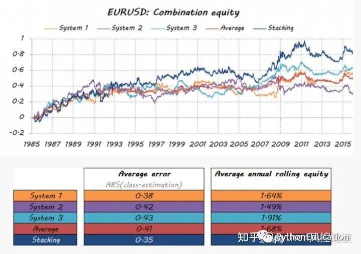
Give an example of stacking to predict the trend of the EURUSD
Imagine that I want to estimate the trend of EURUSD (EUR/USD trend). First, I turned my problem into a classification problem, so I separated the price data into two types (or classes): upward and downward movements. It’s not my intention to second guess every move I make every day. I only want to detect the main trends: long trades up (class = 1) and short trades down (class = 0).
I've done a posteriori split; I mean all historical data is used to decide the classes, so it takes into account some future information. Therefore, I currently cannot ensure iup or down motion. Therefore, an estimate is needed for today's course.
For the purposes of this example, I designed three separate systems. They are three different learners using different sets of attributes. It doesn't matter whether you use the same learner algorithm or they share some/all properties; the point is that they must be different enough to warrant diversity.
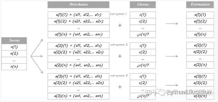
They then trade based on these probabilities: if E is above 50%, it means going long, the larger E. If E is lower than 50%, it is a short entry, the smaller the E.
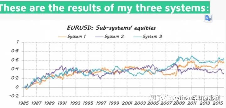
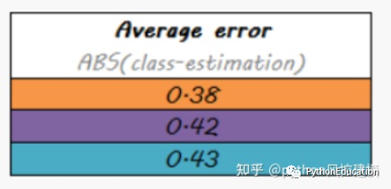
Not ideal, just better than random
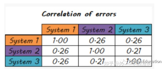
Systematic errors are also less correlated
Can a dream team be formed from a group of weaker players? The purpose of building multiple classifiers is to achieve better predictive performance than any single classifier can achieve. Let's see if this is the case.
The method I will use in this example is based on the Stacking algorithm. The idea of Stacking is that the output of a main classifier called a level 0 model will be used as attributes of another classifier called a meta-model to approximate the same classification problem. The metamodel is left to figure out the merging mechanism. It will be responsible for connecting the reply and true classification of the level 0 model.
The rigorous procedure involves splitting the training set into disjoint sets. Then train each level 0 learner on the entire data, exclude one group, and apply it to the excluded group. By repeating for each group, an estimate of each data is obtained for each learner. These estimates will become the attributes of the trained meta-model or level 1 model. Since my data is a time series, I decided to use the set from day 1 to day d-1 to construct the estimate for day d.
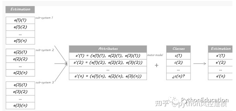
Which mode does this work with? Meta-models can be classification trees, random forests, support vector machines... any classification learner is valid. For this example, I chose to use the nearest neighbor algorithm. This means that the metamodel will estimate the categories of new data to discover similar configurations of class 0 classifications in past data, and will then assign categories to these similar situations.
Let’s see how well my dream team turned out…
The average error value of the stacking model is the lowest
Conclusion This is just one example of the large number of multi-classifiers available. Not only can they help you incorporate part of your solution into a unique answer through modern and original techniques, but they can also create a truly dream team. There is also significant room for improvement in the way individual components are integrated into a system.
So, next time you need a combination, spend a little more time researching the possibilities. Avoid traditional averages and explore more sophisticated approaches through force of habit. They may give you extra performance
Model fusion application in kaggle competition
Model fusion is a very powerful technique that can improve the accuracy of various ML tasks. In this article, I will share my integration method for Kaggle competitions.
For the first part, we look at creating an integration from a commit file. The second part will look at creating ensembles through stacked generalization/hybridization.
I answer why ensemble reduces generalization errors. Finally, I show different integration methods, along with their results and code for you to try yourself. Kaggle Ensembling Guide I answer why ensembles reduce generalization errors. Finally, I show different integration methods, along with their results and code for you to try yourself.
The stacked generation method is a completely different method of combining multiple models. It talks about the concept of combined learners, but it is less used than bagging and boosting. It is not like bagging and boosting, but combines different models. , the specific process is as follows:
1. Divide the training data set into two disjoint sets.
2. Train multiple learners on the first set.
3. Test these learners on the second set.
4. Use the prediction results obtained in the third step as input and the correct response as output to train a high-level learner. What
needs to be paid attention to here is steps 1-3. Effect and cross-validation, we do not use winner-take-all, but use a nonlinear combination learner method

All trained base models will be used to predict the entire training set. The predicted value of the j-th base model for the i-th training sample will be used as the j-th feature value of the i-th sample in the new training set. Finally, based on the new training set for training. In the same way, the prediction process must first go through the predictions of all base models to form a new test set, and finally predict the test set:
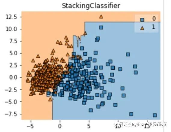
Below we introduce a powerful stacking tool, the mlxtend library, which can quickly stack the sklearn model.
StackingClassifier uses API and parameter analysis:
StackingClassifier(classifiers, meta_classifier, use_probas=False, average_probas=False, verbose=0, use_features_in_secondary=False)
parameter:
classifiers: base classifier, array form, [cl1, cl2, cl3]. The attributes of each base classifier are stored in the class attribute self.clfs_. meta_classifier
: target classifier, which is the classifier that combines the previous classifiers
use_probas: bool (default: False), if set to True, then the input of the target classifier is the category probability value of the previous classification output instead of the category label average_probas: bool (default: False), used to
set the previous parameter when using the probability value output Whether to use the average value when
verbose: int, optional (default=0). Used to control the log output during use. When verbose = 0, nothing is output. When verbose = 1, the serial number and name of the regressor are output. verbose = 2, output detailed parameter information. verbose > 2, automatically set verbose to less than 2, verbose -2.
use_features_in_secondary : bool (default: False). If set to True, the final target classifier will be the data generated by the base classifier and the original data set Train at the same time. If set to False, the final classifier will only be trained using the data produced by the base classifier.
Attributes:
clfs_: attributes of each base classifier, list, shape is [n_classifiers].
meta_clf_: attributes of the final target classifier
method:
fit(X, y)
fit_transform(X, y=None, fit_params)
get_params(deep=True), if the GridSearch method of sklearn is used, then the parameters of the classifier are returned.
predict(X)
predict_proba(X)
score(X, y, sample_weight=None), for a given data set and a given label, return the evaluation accuracy
set_params(params), set the parameters of the classifier, the setting method of params is the same as that of sklearn The format is the same
Part of the actual code of the python fusion model
-
from sklearn.datasets import load_iris -
from mlxtend.classifier import StackingClassifier -
from mlxtend.feature_selection import ColumnSelector -
from sklearn.pipeline import make_pipeline -
from sklearn.linear_model import LogisticRegression -
pipe1 = make_pipeline(ColumnSelector(cols=(0, 2)), -
LogisticRegression()) -
pipe2 = make_pipeline(ColumnSelector(cols=(1, 2, 3)), -
LogisticRegression()) -
sclf = StackingClassifier(classifiers=[pipe1, pipe2], -
meta_classifier=LogisticRegression())
1.1 Basic idea of stacking method
The stacking method is the most popular method in the field of model fusion in recent years. It is not only one of the most commonly used fusion methods by competition champion teams, but also one of the solutions that will be considered when actually implementing artificial intelligence in the industry. As a fusion method of strong learners, Stacking combines the three major advantages of good model effect, strong interpretability, and adaptability to complex data . It is the most practical pioneer method in the field of fusion. Among the many applications of stacking, the practical GBDT+LR stacking in CTR (advertising click-through rate prediction) is particularly famous. Therefore, in the main course of "2022 Machine Learning Practice ", after explaining the common stacking methods, I will explain in detail the usage of GBDT+LR in CTR, and complete a CTR practice.
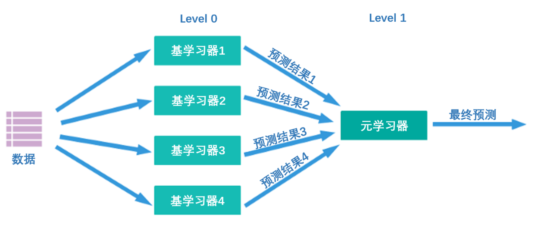
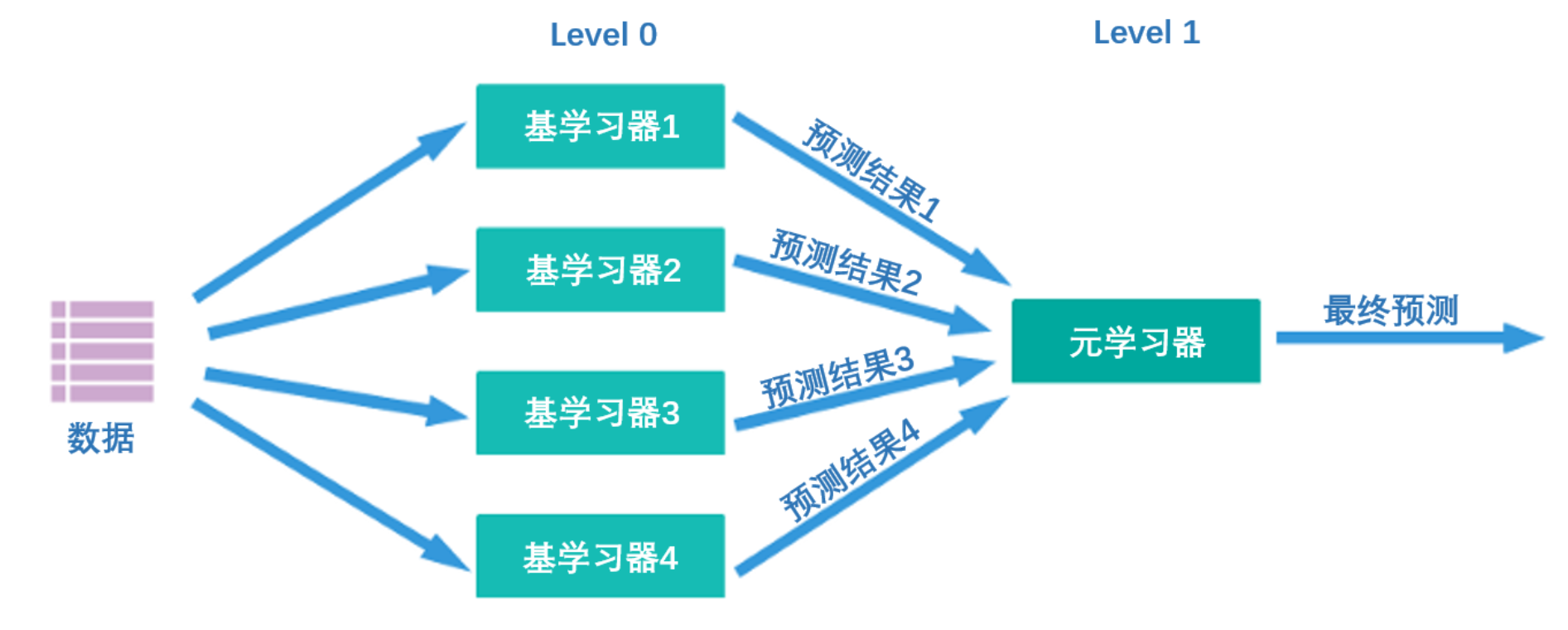
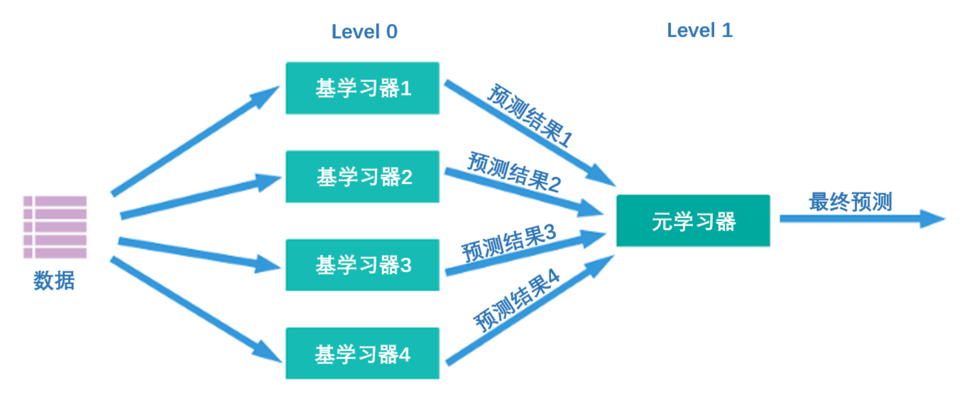
What kind of algorithm is Stacking? Its core idea is actually very simple - first, as shown in the figure below, there are two layers of algorithms in the Stacking structure. The first layer is called level 0, and the second layer is called level 1. Level 0 may contain one or more strong algorithms. Learner, while level 1 can only contain one learner. During training, data will first be input to level 0 for training. After training, each algorithm in level 0 will output corresponding prediction results. We piece together these prediction results into a new feature matrix, and then input it into the level 1 algorithm for training. The final prediction result output by the fusion model is the result output by the level 1 learner.
In this process, the prediction results output by level 0 are generally arranged as follows:
| Learner 1 | Learner 2 | ... | learnern | |
|---|---|---|---|---|
| Sample 1 | xxx | xxx | ... | xxx |
| Sample 2 | xxx | xxx | ... | xxx |
| Sample 3 | xxx | xxx | ... | xxx |
| ... | ... | ... | ... | ... |
| Sample m | xxx | xxx | ... | xxx |
The first column is the result output by learner 1 on all samples, the second column is the result output by learner 2 on all samples, and so on.
At the same time, multiple strong learners trained on level 0 are called base learners (base-model), also called individual learners. The learner trained on level1 is called meta-learner (meta-model). According to industry practice, learners at level 0 are learners with high complexity and strong learning capabilities , such as ensemble algorithms and support vector machines, while learners at level 1 are learners with strong interpretability and relatively simple capabilities , such as Decision trees, linear regression, logistic regression, etc. There is such a requirement because the responsibility of the algorithms at level 0 is to find the relationship between the original data and the label, that is, to establish the hypothesis between the original data and the label, so it requires strong learning capabilities. However, the responsibility of the level 1 algorithm is to fuse the assumptions made by the individual learners and finally output the results of the fusion model, which is equivalent to finding the "best fusion rule" rather than directly establishing assumptions between the original data and labels.
Speaking of which, I wonder if you have noticed that the essence of Stacking is to let the algorithm find out the fusion rules . Although most people may have never been exposed to a series structure similar to the Stacking algorithm, in fact the process of Stacking is completely consistent with the voting method and the averaging method:
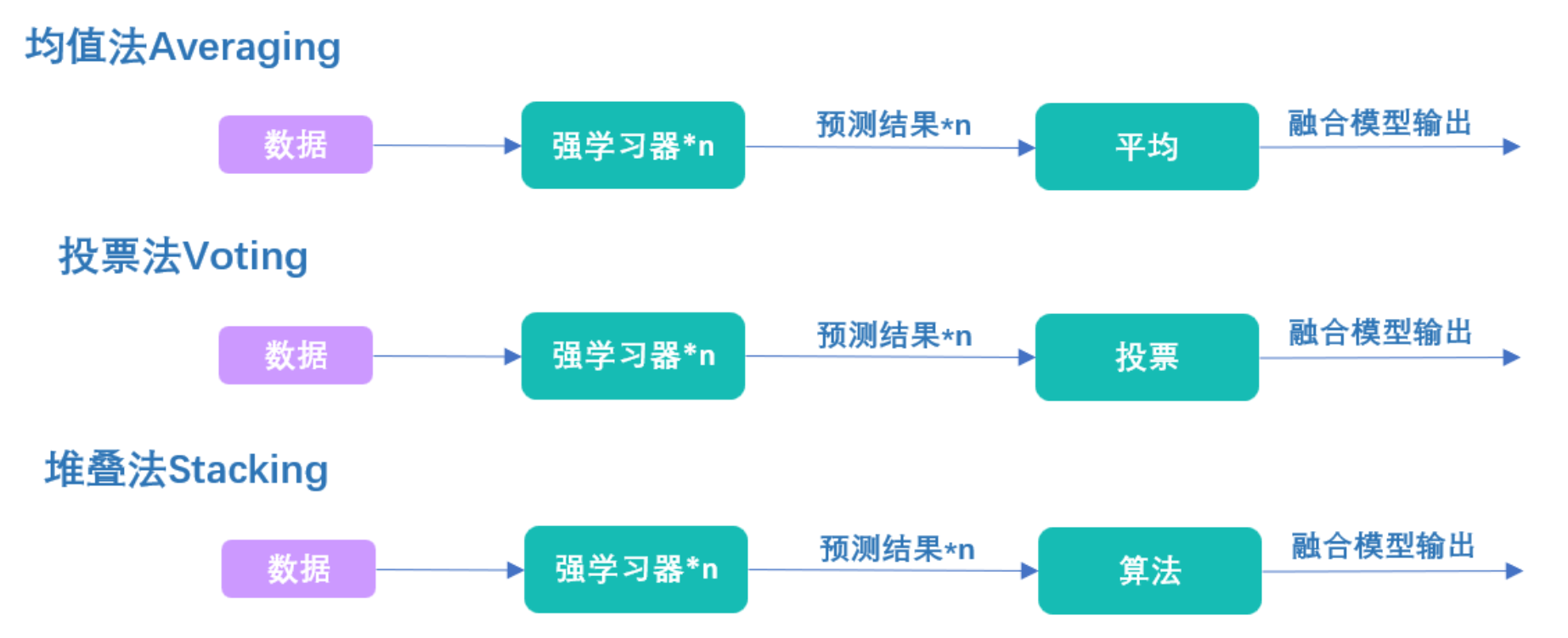
In the voting method, we use voting to fuse the results of strong learners. In the averaging method, we use averaging to fuse the results of strong learners. In the stacking method, we use algorithms to fuse the results of strong learners. When the algorithm on level 1 is linear regression, we are actually solving the weighted sum of all strong learner results, and the process of training linear regression is the process of finding the weight of the weighted sum. Similarly, when the algorithm on level 1 is logistic regression, we are actually solving the weighted sum of all strong learner results, and then applying the sigmoid function based on the sum. The process of training logistic regression is the process of finding the weights of the weighted sum. The same goes for any other simple algorithm.
Although for most algorithms, it is difficult to find a clear name like "weighted sum" to summarize the fusion rules found by the algorithm, but in essence, the level 1 algorithm is just learning how to combine the results output at level 0. Better combined, so Stacking is a method to fuse the results of the learner by training the learner . The averaging method is to average the output results, and the voting method is to vote the output results. The first two are artificially defined fusion methods, but this Stacking is to let the machine help us find the best fusion method. The fundamental advantage of this method is that we can train the meta-learner at level 1 in the direction of minimizing the loss function, while other fusion methods can only guarantee a certain improvement in the fusion results. Therefore Stacking is a more effective method than Voting and Averaging. In practical applications, Stacking often outperforms voting or averaging methods.
After we understand the essence of Stacking, many detailed issues in the implementation process will be easily solved, such as:
- Do you need to perform precise parameter adjustments on the fusion algorithm?
The individual learner is coarse-tuned and the meta-learner is fine-tuned. If the fit is insufficient, both types of learners can be fine-tuned. Theoretically, the closer the algorithm output is to the real label, the better. However, individual learners can easily overfit after being fine-tuned and then fused.
- How to choose the individual learner algorithm to maximize the effect of stacking?
Consistent with voting and averaging, control overfitting, increase diversity, and pay attention to the overall computing time of the algorithm.
- Can the individual learner be a less complex algorithm such as logistic regression or decision tree? Can the meta-learner be a very complex algorithm like xgboost?
All are OK, everything is subject to the model effect. For level 0, when adding weak learners to increase model diversity and the effects of weak learners are better, these algorithms can be retained. For level 1, any algorithm can be used as long as it does not overfit. Personal recommendation is that you can use more complex algorithms for classification, but it is best to use simple algorithms for regression.
- Can level 0 and level 1 algorithms use different loss functions?
Yes, because different loss functions actually measure similar differences: the difference between the true value and the predicted value. However, different losses have different sensitivities to differences, and it is recommended to use similar loss functions if possible.
- Can level 0 and level 1 algorithms use different evaluation metrics?
Personally, it is recommended that algorithms on level 0 and level 1 must use the same model evaluation indicators . Although two groups of algorithms are connected in series in Stacking, the training of these two groups of algorithms is completely separated. In deep learning, we also have a similar structure of powerful algorithms connected in series with weak algorithms. For example, a convolutional neural network consists of a powerful convolutional layer and a weak linear layer connected in series. The main responsibility of the convolutional layer is to find out the relationship between features and labels. The main responsibility of the linear layer is to integrate assumptions and output. However, in deep learning, the training of all layers on a network is performed simultaneously, and the weights on the entire network need to be updated each time the loss function is reduced. However, in Stacking, the algorithm on level 1 does not affect the results of level 0 at all when adjusting the weight. Therefore, in order to ensure that the two groups of algorithms can obtain the results we want after the final fusion, the only evaluation index must be used during training. Baseline for training.
2 Implement stacking in sklearn
class sklearn.ensemble.StackingClassifier(
estimators,
final_estimator=None, *,
cv=None,
stack_method="auto",
n_jobs=None,
passthrough=False,
verbose=0)
class sklearn.ensemble.StackingRegressor(
estimators,
final_estimator=None,*,
cv=None,
n_jobs=None,
passthrough=False,
verbose=0)
| parameter | illustrate |
|---|---|
| estimators | List of individual evaluators. In sklearn, when only using a single evaluator as an individual estimator, the model can run, but the effect is often not very good. |
| final_estimator | A meta-learner can only have one evaluator. When the fusion model performs a classification task, the meta-learner must be a classification algorithm; when the fusion model performs a regression task, the meta-learner must be a regression algorithm. |
| cv | Used to specify the specific type, fold number and other details of cross-validation. You can perform simple K-fold cross-validation or enter the cross-validation class in sklearn. |
| stack_method | Parameters unique to classifiers represent the specific test results output by individual learners. |
| passthrough | When training the meta-learner, whether to add the original data as the feature matrix. |
| n_jobs, verbose | Number of threads and monitoring parameters. |
In sklearn, as long as you enter estimatorsthe sum final_estimator, you can perform stacking. We can continue to use the combination of individual learners used in the voting method and use random forests as meta-learners to complete stacking:
- Tool Library & Data
-
import matplotlib.pyplot as plt -
from sklearn.model_selection import KFold, cross_validate -
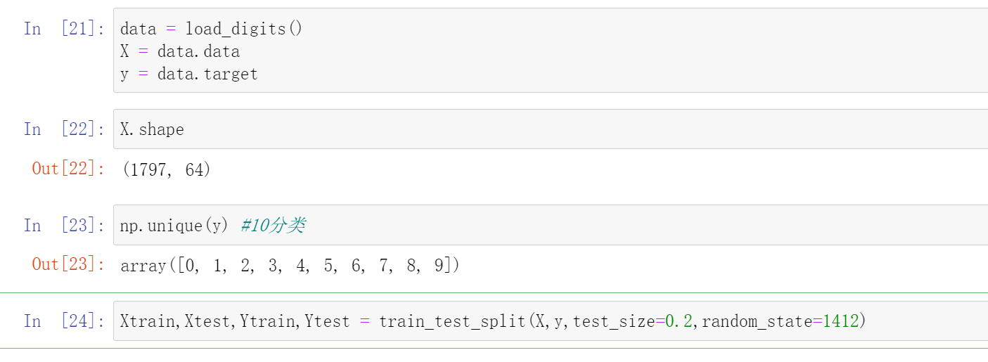
from sklearn.datasets import load_digits #分类 - 手写数字数据集 -
from sklearn.datasets import load_iris -
from sklearn.datasets import load_boston -
from sklearn.model_selection import train_test_split -
from sklearn.neighbors import KNeighborsClassifier as KNNC -
from sklearn.neighbors import KNeighborsRegressor as KNNR -
from sklearn.tree import DecisionTreeRegressor as DTR -
from sklearn.tree import DecisionTreeClassifier as DTC -
from sklearn.linear_model import LinearRegression as LR -
from sklearn.linear_model import LogisticRegression as LogiR -
from sklearn.ensemble import RandomForestRegressor as RFR -
from sklearn.ensemble import RandomForestClassifier as RFC -
from sklearn.ensemble import GradientBoostingRegressor as GBR -
from sklearn.ensemble import GradientBoostingClassifier as GBC -
from sklearn.naive_bayes import GaussianNB -
from sklearn.ensemble import StackingClassifier
-
Xtrain,Xtest,Ytrain,Ytest = train_test_split(X,y,test_size=0.2,random_state=1412)
- Define cross-validation function
-
def fusion_estimators(clf): -
对融合模型做交叉验证,对融合模型的表现进行评估 -
cv = KFold(n_splits=5,shuffle=True,random_state=1412) -
results = cross_validate(clf,Xtrain,Ytrain -
,cv = cv -
,scoring = "accuracy" -
,n_jobs = -1 -
,return_train_score = True -
,verbose=False) -
test = clf.fit(Xtrain,Ytrain).score(Xtest,Ytest) -
print("train_score:{}".format(results["train_score"].mean()) -
cv_mean:{}".format(results["test_score"].mean()) -
test_score:{}".format(test)
-
def individual_estimators(estimators): -
对模型融合中每个评估器做交叉验证,对单一评估器的表现进行评估 -
for estimator in estimators: -
cv = KFold(n_splits=5,shuffle=True,random_state=1412) -
results = cross_validate(estimator[1],Xtrain,Ytrain -
,cv = cv -
,scoring = "accuracy" -
,n_jobs = -1 -
,return_train_score = True -
,verbose=False) -
test = estimator[1].fit(Xtrain,Ytrain).score(Xtest,Ytest) -
print(estimator[0] -
train_score:{}".format(results["train_score"].mean()) -
cv_mean:{}".format(results["test_score"].mean()) -
test_score:{}".format(test)
- Definition of individual learners and meta-learners
When we explained the voting method before, we have given a detailed explanation on how to define individual learners, and have also made a lot of efforts to find the following 7 models. Here, we will use the 7 models selected from Voting:
-
clf1 = LogiR(max_iter = 3000, C=0.1, random_state=1412,n_jobs=8) -
clf2 = RFC(n_estimators= 100,max_features="sqrt",max_samples=0.9, random_state=1412,n_jobs=8) -
clf3 = GBC(n_estimators= 100,max_features=16,random_state=1412) -
clf4 = DTC(max_depth=8,random_state=1412) -
clf5 = KNNC(n_neighbors=10,n_jobs=8) -
clf7 = RFC(n_estimators= 100,max_features="sqrt",max_samples=0.9, random_state=4869,n_jobs=8) -
clf8 = GBC(n_estimators= 100,max_features=16,random_state=4869) -
estimators = [("Logistic Regression",clf1), ("RandomForest", clf2) -
, ("GBDT",clf3), ("Decision Tree", clf4), ("KNN",clf5) -
#, ("Bayes",clf6) -
, ("RandomForest2", clf7), ("GBDT2", clf8)
- Import sklearn for modeling
-
final_estimator = RFC(n_estimators=100 -
, min_impurity_decrease=0.0025 -
, random_state= 420, n_jobs=8) -
clf = StackingClassifier(estimators=estimators #level0的7个体学习器 -
,final_estimator=final_estimator #level 1的元学习器 -
,n_jobs=8)
Before adjusting the fitting: that is, without adding min_impurity_decrease=0.0025
-
fusion_estimators(clf) #没有过拟合限制 -
cv_mean:0.9812112853271389 -
test_score:0.9861111111111112
After adding overfitting
-
fusion_estimators(clf) #精调过拟合 -
cv_mean:0.9812185443283005 -
test_score:0.9888888888888889
| benchmark | voting laws | stacking method | |
|---|---|---|---|
| 5 fold cross validation | 0.9666 | 0.9833 | 0.9812(↓) |
| Test set results | 0.9527 | 0.9889 | 0.9889(-) |
It can be seen that the score of stacking on the test set is the same as the voting method, but the 5-fold cross-validation score is not as high as the voting method. This may be because the data we train now is relatively simple, but when the data learning is more difficult, the advantages of stacking will slowly emerge. Of course, the meta-learner we are using now has almost default parameters. We can use Bayesian optimization to fine-tune the parameters of the meta-learner, and then compare them. The effect of the stacking method may surpass the voting method.
Feature matrix of 3-element learner
3.1 Two issues with meta-learner feature matrices
In the stacking process, individual learners train and predict on the original data, and then arrange the prediction results into a new feature matrix and put them into the meta-learner for learning. Among them, the prediction results of individual learners, that is, the matrix that needs to be trained by the meta-learner, are generally arranged as follows:
| Learner 1 | Learner 2 | ... | learnern | |
|---|---|---|---|---|
| Sample 1 | xxx | xxx | ... | xxx |
| Sample 2 | xxx | xxx | ... | xxx |
| Sample 3 | xxx | xxx | ... | xxx |
| ... | ... | ... | ... | ... |
| Sample m | xxx | xxx | ... | xxx |
Based on our understanding of machine learning and model fusion, it is not difficult to find the following two problems:
- First, there must be very few features in the feature matrix of the meta-learner
An individual learner can only output one set of prediction results. We arrange these prediction results, and the number of features in the new feature matrix is equal to the number of individual learners. Generally, there are at most 20-30 individual learners in the fusion model, which means that there are at most 20-30 features in the feature matrix of the meta-learner. This feature quantity is far from enough for machine learning algorithms in industry and competitions.
- Secondly, there are not too many samples in the feature matrix of the meta-learner.
The responsibility of the individual learner is to find the hypothesis between the original data and the label. In order to verify whether this hypothesis is accurate, what we need to look at is the generalization ability of the individual learner. Only when the generalization ability of the individual learner is strong, can we safely put the prediction results output by the individual learner into the meta-learner for fusion.
However. When we train the stacking model, we must divide the original data set into three parts: training set, verification set and test set - the
test set is used to test the effect of the entire fusion model, so it cannot be used during the training process.
The training set is used to train individual learners, and it is content that has been fully disclosed to the individual learners. If predictions are made on the training set, the prediction results will be "high" and cannot represent the generalization ability of the individual learners.
Therefore, in the end, only a small verification set is left that can be used for prediction and represents the true learning level of the individual learner . Generally, the verification set only accounts for 30%-40% of the entire data set at most, which means that the sample size in the feature matrix used by the meta-learner is at most 40% of the original data.
It is no wonder that in industry practice, the meta-learner needs to be a less complex algorithm, because the feature matrix of the meta-learner is far smaller than the standards required by industrial machine learning in terms of feature volume and sample size. In order to solve these two problems, there are multiple solutions in the Stacking method, and these solutions can be implemented through the stacking class in sklearn.
class sklearn.ensemble.StackingClassifier(estimators, final_estimator=None, *, cv=None, stack_method="auto", n_jobs=None, passthrough=False, verbose=0)
class sklearn.ensemble.StackingRegressor(estimators, final_estimator=None, *, cv=None, n_jobs=None, passthrough=False, verbose=0)
| parameter | illustrate |
|---|---|
| estimators | List of individual evaluators. In sklearn, when only using a single evaluator as an individual estimator, the model can run, but the effect is often not very good. |
| final_estimator | A meta-learner can only have one evaluator. When the fusion model performs a classification task, the meta-learner must be a classification algorithm; when the fusion model performs a regression task, the meta-learner must be a regression algorithm. |
| cv | Used to specify the specific type, fold number and other details of cross-validation. You can perform simple K-fold cross-validation or enter the cross-validation class in sklearn. |
| stack_method | Parameters unique to classifiers represent the specific test results output by individual learners. |
| passthrough | When training the meta-learner, whether to add the original data as the feature matrix. |
| n_jobs, verbose | Number of threads and monitoring parameters. |
3.2 Solution to too small sample size: cross-validation
- 参数
cv,在stacking中执行交叉验证
在stacking方法被提出的原始论文当中,原作者自然也意识到了元学习器的特征矩阵样本量太少这个问题,因此提出了在stacking流程内部使用交叉验证来扩充元学习器特征矩阵的想法,即在内部对每个个体学习器做交叉验证,但并不用这个交叉验证的结果来验证泛化能力,而是直接把交叉验证当成了生产数据的工具。
具体的来看,在stacking过程中,我们是这样执行交叉验证的——
对任意个体学习器来说,假设我们执行5折交叉验证,我们会将训练数据分成5份,并按照4份训练、1份验证的方式总共建立5个模型,训练5次:
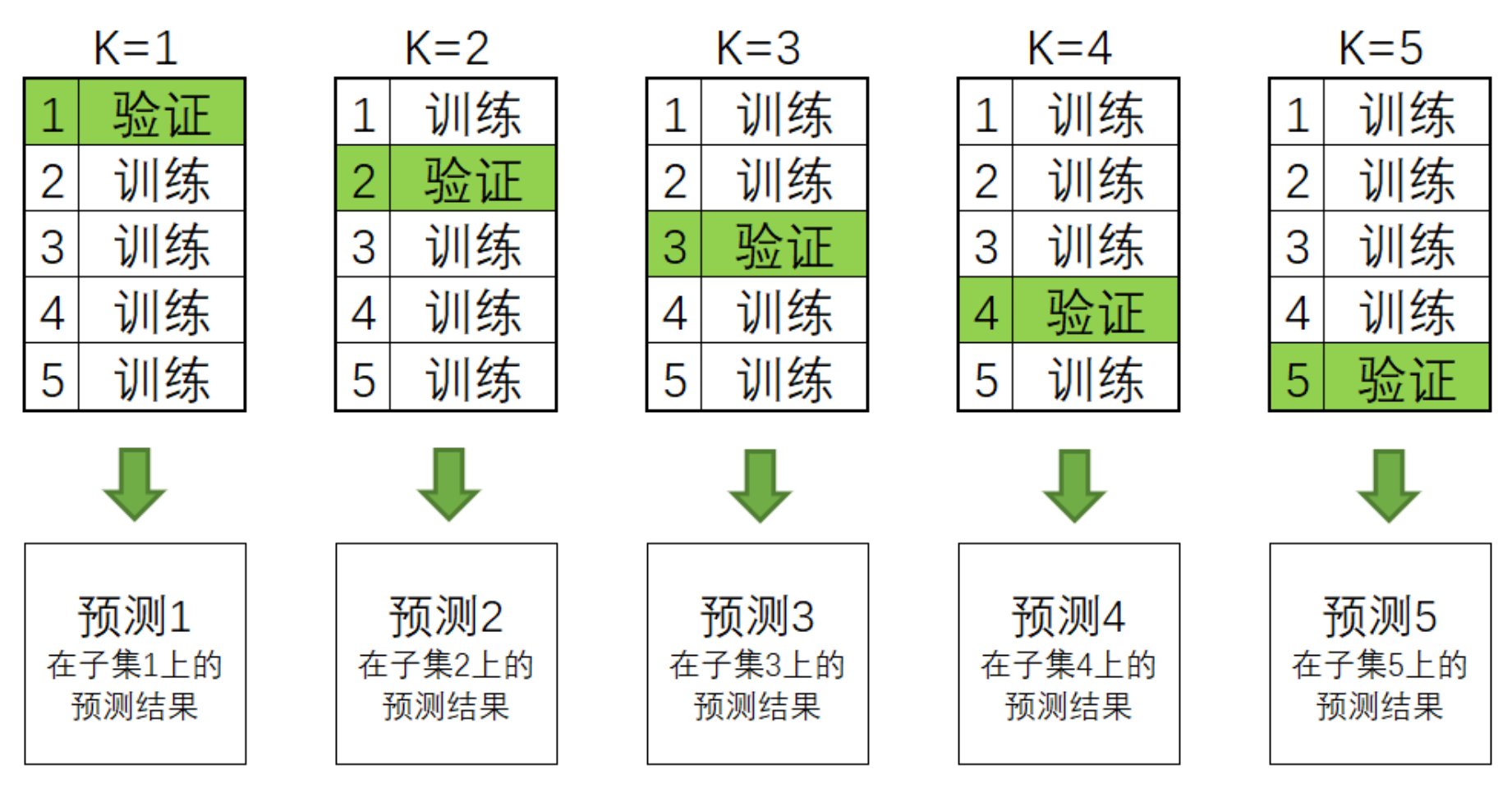
在交叉验证过程中,每次验证集中的数据都是没有被放入模型进行训练的,因此这些验证集上的预测结果都可以衡量模型的泛化能力。
一般来说,交叉验证的最终输出是5个验证集上的分数,但计算分数之前我们一定是在5个验证集上分别进行预测,并输出了结果。所以我们可以在交叉验证中建立5个模型,轮流得到5个模型输出的预测结果,而这5个预测结果刚好对应全数据集中分割的5个子集。这是说,我们完成交叉验证的同时,也对原始数据中全部的数据完成了预测。现在,只要将5个子集的预测结果纵向堆叠,就可以得到一个和原始数据中的样本一一对应的预测结果。这种纵向堆叠正像我们在海滩上堆石子(stacking)一样,这也是“堆叠法”这个名字的由来。

用这样的方法来进行预测,可以让任意个体学习器输出的预测值数量 = 样本量,如此,元学习器的特征矩阵的行数也就等于原始数据的样本量了:
| 学习器1 | 学习器2 | ... | 学习器n | |
|---|---|---|---|---|
| 样本1 | xxx | xxx | ... | xxx |
| 样本2 | xxx | xxx | ... | xxx |
| 样本3 | xxx | xxx | ... | xxx |
| ... | ... | ... | ... | ... |
| 样本m | xxx | xxx | ... | xxx |
在stacking过程中,这个交叉验证流程是一定会发生的,不属于我们可以人为干涉的范畴。不过,我们可以使用参数cv来决定具体要使用怎样的交叉验证,包括具体使用几折验证,是否考虑分类标签的分布等等。具体来说,参数cv中可以输入:
输入None,默认使用5折交叉验证
输入sklearn中任意交叉验证对象
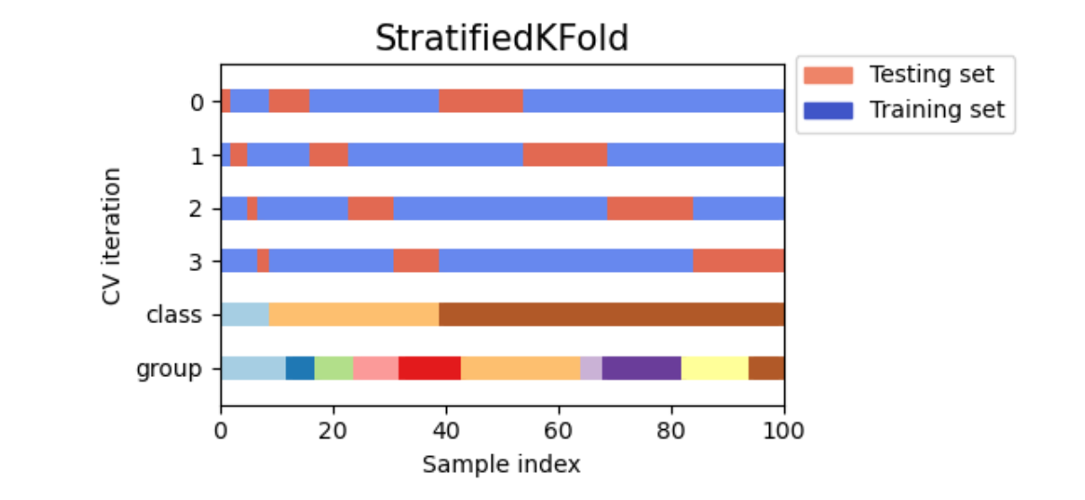
输入任意整数,表示在Stratified K折验证中的折数。Stratified K折验证是会考虑标签中每个类别占比的交叉验证,如果选择Stratified K折交叉验证,那每次训练时交叉验证会保证原始标签中的类别比例 = 训练标签的类别比例 = 验证标签的类别比例。
现在你知道Stacking是如何处理元学习器的特征矩阵样本太少的问题了。需要再次强调的是,内部交叉验证的并不是在验证泛化能力,而是一个生产数据的工具,因此交叉验证本身没有太多可以调整的地方。唯一值得一提的是,当交叉验证的折数较大时,模型的抗体过拟合能力会上升、同时学习能力会略有下降。当交叉验证的折数很小时,模型更容易过拟合。但如果数据量足够大,那使用过多的交叉验证折数并不会带来好处,反而只会让训练时间增加而已:
-
estimators = [("Logistic Regression",clf1), ("RandomForest", clf2) -
, ("GBDT",clf3), ("Decision Tree", clf4), ("KNN",clf5) -
#, ("Bayes",clf6) -
, ("RandomForest2", clf7), ("GBDT2", clf8) -
final_estimator = RFC(n_estimators=100 -
, min_impurity_decrease=0.0025 -
, random_state= 420, n_jobs=8)
-
clf = StackingClassifier(estimators=estimators -
,final_estimator=final_estimator -
, cv = cv -
, n_jobs=8) -
clf.fit(Xtrain,Ytrain) -
print((time.time() - start)) #消耗时间 -
print(clf.score(Xtrain,Ytrain)) #训练集上的结果 -
print(clf.score(Xtest,Ytest)) #测试集上的结果
可以看到,随着cv中折数的上升,训练时间一定会上升,但是模型的表现却不一定。因此,选择5~10折交叉验证即可。同时,由于stacking当中自带交叉验证,又有元学习器这个算法,因此堆叠法的运行速度是比投票法、均值法缓慢很多的,这是stacking堆叠法不太人性化的地方。
3.3 特征太少的解决方案
- 参数
stack_method,更换个体学习器输出的结果类型
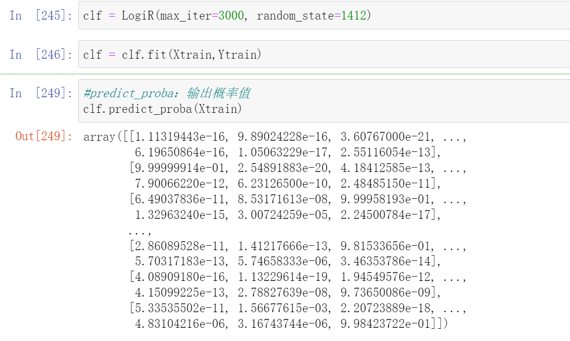
对于分类stacking来说,如果特征量太少,我们可以更换个体学习器输出的结果类型。具体来说,如果个体学习器输出的是具体类别(如[0,1,2]),那1个个体学习器的确只能输出一列预测结果。但如果把输出的结果类型更换成概率值、置信度等内容,输出结果的结构一下就可以从一列拓展到多列。
如果这个行为由参数stack_method控制,这是只有StackingClassifier才拥有的参数,它控制个体分类器具体的输出。stack_method里面可以输入四种字符串:"auto", "predict_proba", "decision_function", "predict",除了"auto"之外其他三个都是sklearn常见的接口。
-
clf = LogiR(max_iter=3000, random_state=1412) -
clf = clf.fit(Xtrain,Ytrain)
-
clf.predict_proba(Xtrain)
-
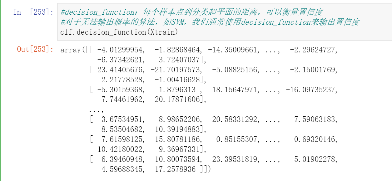
#decision_function:每个样本点到分类超平面的距离,可以衡量置信度 -
#对于无法输出概率的算法,如SVM,我们通常使用decision_function来输出置信度 -
clf.decision_function(Xtrain)
对参数stack_method有:
输入"auto",sklearn会在每个个体学习器上按照"predict_proba", "decision_function", "predict"的顺序,分别尝试学习器可以使用哪个接口进行输出。即,如果一个算法可以使用predict_proba接口,那就不再尝试后面两个接口,如果无法使用predict_proba,就尝试能否使用decision_function。
输入三大接口中的任意一个接口名,则默认全部个体学习器都按照这一接口进行输出。然而,如果遇见某个算法无法按照选定的接口进行输出,stacking就会报错。
因此,我们一般都默认让stack_method保持为"auto"。从上面的我们在逻辑回归上尝试的三个接口结果来看,很明显,当我们把输出的结果类型更换成概率值、置信度等内容,输出结果的结构一下就可以从一列拓展到多列。
- predict_proba
对二分类,输出样本的真实标签1的概率,一列
对n分类,输出样本的真实标签为[0,1,2,3...n]的概率,一共n列
- decision_function
对二分类,输出样本的真实标签为1的置信度,一列
对n分类,输出样本的真实标签为[0,1,2,3...n]的置信度,一共n列
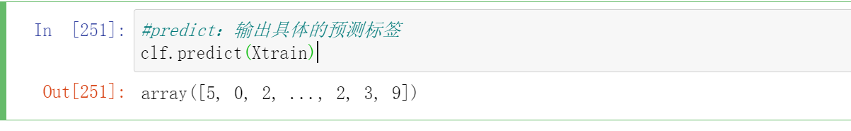
- predict
对任意分类形式,输出算法在样本上的预测标签,一列
在实践当中,我们会发现输出概率/置信度的效果比直接输出预测标签的效果好很多,既可以向元学习器提供更多的特征、还可以向元学习器提供个体学习器的置信度。我们在投票法中发现使用概率的“软投票”比使用标签类被的“硬投票”更有效,也是因为考虑了置信度。
- 参数
passthrough,将原始特征矩阵加入新特征矩阵
对于分类算法,我们可以使用stack_method,但是对于回归类算法,我们没有这么多可以选择的接口。回归类算法的输出永远就只有一列连续值,因而我们可以考虑将原始特征矩阵加入个体学习器的预测值,构成新特征矩阵。这样的话,元学习器所使用的特征也不会过于少了。当然,这个操作有较高的过拟合风险,因此当特征过于少、且stacking算法的效果的确不太好的时候,我们才会考虑这个方案。
控制是否将原始数据加入特征矩阵的参数是passthrough,我们可以在该参数中输入布尔值。当设置为False时,表示不将原始特征矩阵加入个体学习器的预测值,设置为True时,则将原始特征矩阵加入个体学习器的预测值、构成大特征矩阵。
- 接口
transform与属性stack_method_
-
estimators = [("Logistic Regression",clf1), ("RandomForest", clf2) -
, ("GBDT",clf3), ("Decision Tree", clf4), ("KNN",clf5) -
#, ("Bayes",clf6) -
, ("RandomForest2", clf7), ("GBDT2", clf8)
-
final_estimator = RFC(n_estimators=100 -
, min_impurity_decrease=0.0025 -
, random_state= 420, n_jobs=8) -
clf = StackingClassifier(estimators=estimators -
,final_estimator=final_estimator -
,stack_method = "auto" -
,n_jobs=8)
clf = clf.fit(Xtrain,Ytrain)
当我们训练完毕stacking算法后,可以使用接口transform来查看当前元学习器所使用的训练特征矩阵的结构:
-
clf.transform(Xtrain).shape
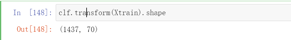
这个70 代表这个一共有7个个体学习器,每个个体学习器都有10个概率输出
如之前所说,这个特征矩阵的行数就等于训练的样本量:
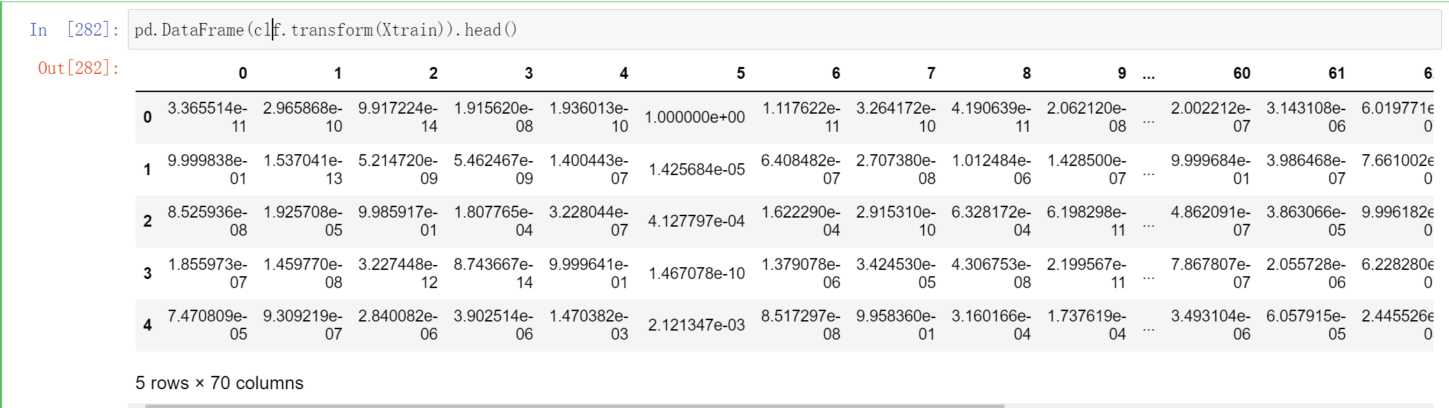
不过你能判断为什么这里有70列吗?因为我们有7个个体学习器,而现在数据是10分类的数据,因此每个个体学习器都输出了类别[0,1,2,3,4,5,6,7,8,9]所对应的概率,因此总共产出了70列数据:
pd.DataFrame(clf.transform(Xtrain)).head()
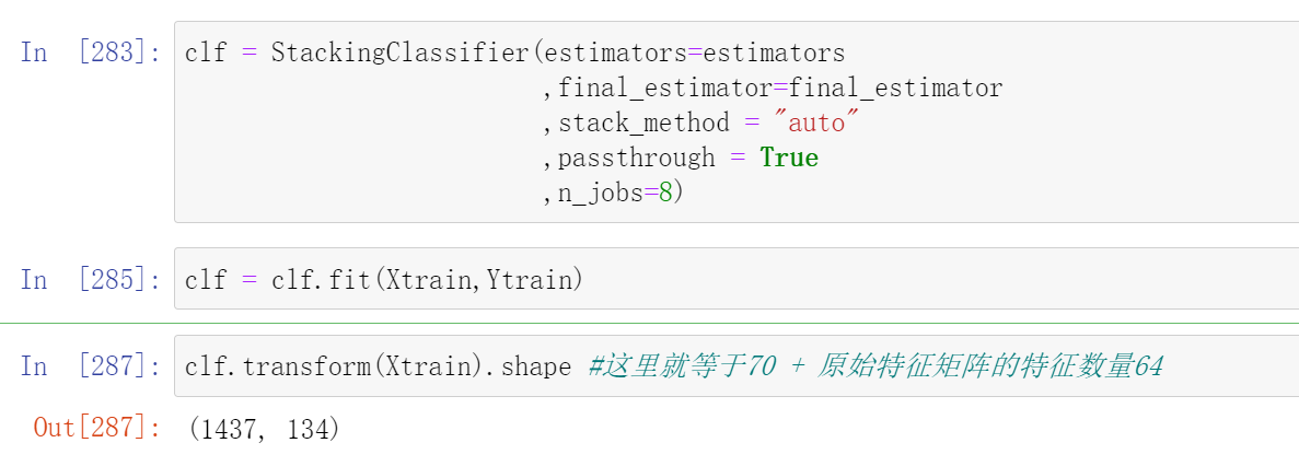
如果加入参数passthrough,特征矩阵的特征量会变得更大:
-
clf = StackingClassifier(estimators=estimators -
,final_estimator=final_estimator -
,stack_method = "auto" -
,passthrough = True -
,n_jobs=8)
clf = clf.fit(Xtrain,Ytrain)
-
clf.transform(Xtrain).shape #这里就等于70 + 原始特征矩阵的特征数量64
使用属性stack_method_,我们可以查看现在每个个体学习器都使用了什么接口做为预测输出:
clf.stack_method_
["predict_proba",
"predict_proba",
"predict_proba",
"predict_proba",
"predict_proba",
"predict_proba",
"predict_proba"]
不难发现,7个个体学习器都使用了predict_proba的概率接口进行输出,这与我们选择的算法都是可以输出概率的算法有很大的关系
4 Stacking融合的训练/测试流程
现在我们已经知道了stacking算法中所有关于训练的信息,我们可以梳理出如下训练流程:
- stacking的训练
- 将数据分割为训练集、测试集,其中训练集上的样本为(M_{train}),测试集上的样本量为(M_{test})
- 将训练集输入level 0的个体学习器,分别在每个个体学习器上进行交叉验证。在每个个体学习器上,将所有交叉验证的验证结果纵向堆叠形成预测结果。假设预测结果为概率值,当融合模型执行回归或二分类任务时,该预测结果的结构为((M_{train},1)),当融合模型执行K分类任务时(K>2),该预测结果的结构为((M_{train},K))
- 将所有个体学习器的预测结果横向拼接,形成新特征矩阵。假设共有N个个体学习器,则新特征矩阵的结构为((M_{train}, N))。如果是输出多分类的概率,那最终得出的新特征矩阵的结构为((M_{train}, N*K))
- 将新特征矩阵放入元学习器进行训练。
不难发现,虽然训练的流程看起来比较流畅,但是测试却不知道从何做起,因为:
-
最终输出预测结果的是元学习器,因此直觉上来说测试数据集或许应该被输入到元学习器当中。然而,元学习器是使用新特征矩阵进行预测的,新特征矩阵的结构与规律都与原始数据不同,所以元学习器根本不可能接受从原始数据中分割出来的测试数据。因此正确的做法应该是让测试集输入level 0的个体学习器。
-
然而,这又存在问题了:level 0的个体学习器们在训练过程中做的是交叉验证,而交叉验证只会输出验证结果,不会留下被训练的模型。因此在level 0中没有可以用于预测的、已经训练完毕的模型。
为了解决这个矛盾在我们的训练流程中,存在着隐藏的步骤:
- stacking的训练
- 将数据分割为训练集、测试集,其中训练集上的样本为(M_{train}),测试集上的样本量为(M_{test})
- 将训练集输入level 0的个体学习器,分别在每个个体学习器上进行交叉验证。在每个个体学习器上,将所有交叉验证的验证结果纵向堆叠形成预测结果。假设预测结果为概率值,当融合模型执行回归或二分类任务时,该预测结果的结构为((M_{train},1)),当融合模型执行K分类任务时(K>2),该预测结果的结构为((M_{train},K))
- 隐藏步骤:使用全部训练数据对所有个体学习器进行训练,为测试做好准备。
- 将所有个体学习器的预测结果横向拼接,形成新特征矩阵。假设共有N个个体学习器,则新特征矩阵的结构为((M_{train}, N)).
- 将新特征矩阵放入元学习器进行训练。
- stacking的测试
- 将测试集输入level0的个体学习器,分别在每个个体学习器上预测出相应结果。假设测试结果为概率值,当融合模型执行回归或二分类任务时,该测试结果的结构为((M_{test},1)),当融合模型执行K分类任务时(K>2),该测试结果的结构为((M_{test},K))
- 将所有个体学习器的预测结果横向拼接为新特征矩阵。假设共有N个个体学习器,则新特征矩阵的结构为((M_{test}, N)).
- 将新特征矩阵放入元学习器进行预测。
因此在stacking中,不仅要对个体学习器完成全部交叉验证,还需要在交叉验证结束后,重新使用训练数据来训练所有的模型。无怪Stacking融合的复杂度较高、并且运行缓慢了。
到现在,我们已经讲解完毕投票法和堆叠法了。在sklearn中,我们讲解了下面4个类:
| 融合方法 | 类 |
|---|---|
| 投票法 | ensemble.VotingClassifier |
| 平均法 | ensemble.VotingRegressor |
| 堆叠法分类 | ensemble.StackingClassifier |
| 堆叠法回归 | ensemble.StackingRegressor |
虽然这些类是模型融合方法,但我们可以像使用任意单一算法类一样任意地使用这些方法——我们可以很轻松地对这些类执行手动调参、交叉验证、网格搜索、贝叶斯优化、管道打包等操作,而无需担心代码的兼容问题。但需要注意的是,sklearn中的融合工具只支持sklearn中的评估器,不支持xgb、lgbm的原生代码。因此,如果我们想要对原生代码下的模型进行融合,必须自己手写融合过程。
二 改进后的堆叠法:Blending
1 Blending的基本思想与流程
Blending融合是在Stacking融合的基础上改进过后的算法。在之前的课程中我们提到,堆叠法stacking在level1上使用算法,这可以令融合本身向着损失函数最小化的方向进行,同时stacking使用自带的内部交叉验证来生成数据,可以深度使用训练数据,让模型整体的效果更好。但在这些操作的背后,存在两个巨大的问题:
-
stacking融合需要巨大的计算量,需要的时间和算力成本较高,以及
-
stacking融合在数据和算法上都过于复杂,因此融合模型过拟合的可能性太高。
针对stacking存在的这两个问题,竞赛冠军队们持续探索,并且在实践过程中创造了多种改进的stacking方法。今天,多种stacking方法中较为有效的方法之一就是著名的Blending方法。Blending直译为“混合”,但它的核心思路其实与Stacking完全一致:使用两层算法串联,level0上存在多个强学习器,level1上有且只有一个元学习器,且level0上的强学习器负责拟合数据与真实标签之间的关系、并输出预测结果、组成新的特征矩阵,然后让level1上的元学习器在新的特征矩阵上学习并预测。
然而,与stacking不同的是,为了降低计算量、降低融合模型过拟合风险,Blending取消了K折交叉验证、并且大大地降低了元学习器所需要训练的数据量,其具体流程如下:
- blending的训练
- 将数据分割为训练集、验证集与测试集,其中训练集上的样本为(M_{train}),验证集上的样本为(M_v),测试集上的样本量为(M_{test})
- 将训练集输入level 0的个体学习器,分别在每个个体学习器上训练。训练完毕后,在验证集上进行验证,输出验证集上的预测结果。假设预测结果为概率值,当融合模型执行回归或二分类任务时,该预测结果的结构为((M_v,1)),当融合模型执行K分类任务时(K>2),该预测结果的结构为((M_v,K))。此时此刻,所有个体学习器都被训练完毕了。
- 将所有个体学习器的验证结果横向拼接,形成新特征矩阵。假设共有N个个体学习器,则新特征矩阵的结构为((M_v, N))。
- 将新特征矩阵放入元学习器进行训练。
- blending的测试
- 将测试集输入level0的个体学习器,分别在每个个体学习器上预测出相应结果。假设测试结果为概率值,当融合模型执行回归或二分类任务时,该测试结果的结构为((M_{test},1)),当融合模型执行K分类任务时(K>2),该测试结果的结构为((M_{test},K))
- 将所有个体学习器的预测结果横向拼接为新特征矩阵。假设共有N个个体学习器,则新特征矩阵的结构为((M_{test}, N)).
- 将新特征矩阵放入元学习器进行预
测。
2 手动实现Blending算法
-
def BlendingClassifier(X,y,estimators,final_estimator,test_size=0.2,vali_size=0.4): -
X,y:整体数据集,会被分割为训练集、测试集、验证集三部分 -
estimators: level0的个体学习器,输入格式形如sklearn中要求的[(名字,算法),(名字,算法)...] -
test_size:测试集占全数据集的比例 -
vali_size:验证集站全数据集的比例 -
#2.分训练和验证集,验证集占完整数据集的比例为0.4,因此占排除测试集之后的比例为0.4/(1-0.2) -
X_,Xtest,y_,Ytest = train_test_split(X,y,test_size=test_size,random_state=1412) -
Xtrain,Xvali,Ytrain,Yvali = train_test_split(X_,y_,test_size=vali_size/(1-test_size),random_state=1412) -
#建立空dataframe用于保存个体学习器上的验证结果,即用于生成新特征矩阵 -
#新建空列表用于保存训练完毕的个体学习器,以便在测试中使用 -
NewX_vali = pd.DataFrame() -
trained_estimators = [] -
#循环、训练每个个体学习器、并收集个体学习器在验证集上输出的概率 -
for clf_id, clf in estimators: -
clf = clf.fit(Xtrain,Ytrain) -
val_predictions = pd.DataFrame(clf.predict_proba(Xvali)) -
#保存结果,在循环中逐渐构筑新特征矩阵 -
NewX_vali = pd.concat([NewX_vali,val_predictions],axis=1) -
trained_estimators.append((clf_id,clf)) -
#元学习器在新特征矩阵上训练、并输出训练分数 -
final_estimator = final_estimator.fit(NewX_vali,Yvali) -
train_score = final_estimator.score(NewX_vali,Yvali) -
#建立空dataframe用于保存个体学习器上的预测结果,即用于生成新特征矩阵 -
NewX_test = pd.DataFrame() -
#循环,在每个训练完毕的个体学习器上进行预测,并收集每个个体学习器上输出的概率 -
for clf_id,clf in trained_estimators: -
test_prediction = pd.DataFrame(clf.predict_proba(Xtest)) -
#保存结果,在循环中逐渐构筑特征矩阵 -
NewX_test = pd.concat([NewX_test,test_prediction],axis=1) -
#元学习器在新特征矩阵上测试、并输出测试分数 -
test_score = final_estimator.score(NewX_test,Ytest) -
print(train_score,test_score)
-
clf1 = LogiR(max_iter = 3000, C=0.1, random_state=1412,n_jobs=8) -
clf2 = RFC(n_estimators= 100,max_features="sqrt",max_samples=0.9, random_state=1412,n_jobs=8) -
clf3 = GBC(n_estimators= 100,max_features=16,random_state=1412) -
clf4 = DTC(max_depth=8,random_state=1412) -
clf5 = KNNC(n_neighbors=10,n_jobs=8) -
clf7 = RFC(n_estimators= 100,max_features="sqrt",max_samples=0.9, random_state=4869,n_jobs=8) -
clf8 = GBC(n_estimators= 100,max_features=16,random_state=4869) -
estimators = [("Logistic Regression",clf1), ("RandomForest", clf2) -
, ("GBDT",clf3), ("Decision Tree", clf4), ("KNN",clf5) -
#, ("Bayes",clf6) -
#, ("RandomForest2", clf7), ("GBDT2", clf8)
-
final_estimator = RFC(n_estimators= 100 -
#, max_depth = 8 -
, min_impurity_decrease=0.0025 -
, random_state= 420, n_jobs=8)
-
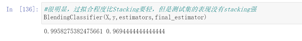
#很明显,过拟合程度比Stacking要轻,但是测试集的表现没有stacking强 -
BlendingClassifier(X,y,estimators,final_estimator)
-
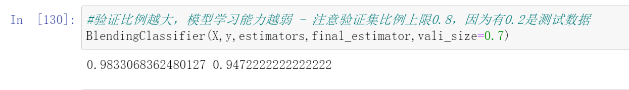
#验证比例越大,模型学习能力越弱 - 注意验证集比例上限0.8,因为有0.2是测试数据 -
BlendingClassifier(X,y,estimators,final_estimator,vali_size=0.7)
-
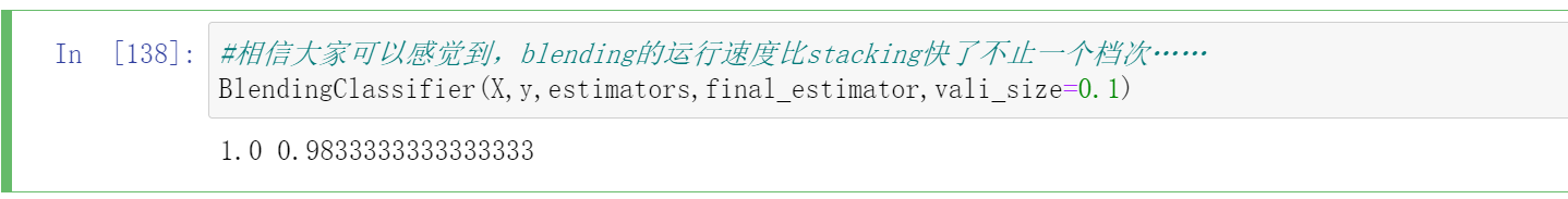
#blending的运行速度比stacking快了不止一个档次…… -
BlendingClassifier(X,y,estimators,final_estimator,vali_size=0.1)
| benchmark | 投票法 | Stacking | Blending | |
|---|---|---|---|---|
| 5折交叉验证 | 0.9666 | 0.9833 | 0.9812(↓) | - |
| 测试集结果 | 0.9527 | 0.9889 | 0.9889(-) | 0.9833(↓) |
从结果来看,投票法表现最稳定和优异,这与我们选择的数据集是较为简单的数据集有关,同时投票法也是我们调整最多、最到位的算法。在大型数据集上运行时,stacking和blending会展现出更多的优势。到这里我们的blending就讲解完毕了,在《2022机器学习实战》正式课程当中,我们将会更详细地讲解Blending在xgboost等复杂算法上的应用。
参考:https://www.cnblogs.com/lipu123/p/17563377.html
For more knowledge about python machine learning, please follow the official account (python risk control model)