Note: This article has made some modifications based on the previous article, and the repeated parts can be skipped. An example project is the task of classifying cancer cells based on the LR model.
With the advent of the era of artificial intelligence, machine learning has become a key tool for solving problems, such as identifying whether a transaction is fraudulent, predicting rainfall, categorizing news, and recommending product marketing. We next describe in detail how machine learning is applied to practical problems, and outline the general flow of machine learning applications.
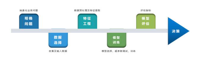
1.1 Define the problem
Clarifying the business problem is a prerequisite for machine learning, that is, abstracting the problem as a machine learning prediction problem: what kind of data needs to be learned as input, and what kind of model to make decisions as the goal is to get as output.
A simple news classification scenario is to learn the existing news and its category label data, obtain a text classification model, and use the model to predict the category of new news every day, so as to classify it into each news channel.

Technology Exchange
Technology must learn to share and communicate, and it is not recommended to work behind closed doors. One person can go fast, and a group of people can go farther.
Good articles are inseparable from the sharing and recommendation of fans, dry data, data sharing, data, and technical exchange improvement, all of which can be obtained by adding the communication group. The group has more than 2,000 friends. The best way to add notes is: source + interest directions, making it easy to find like-minded friends.
Method ①, add WeChat account: dkl88191, remarks: from CSDN + python
method ②, WeChat search official account: Python learning and data mining, background reply: add group
1.2 Data Selection
There is a widely circulated saying in machine learning: "Data and features determine the upper limit of machine learning results, and the model algorithm is only as close as possible to this upper limit", which means that the quality of data and its feature representation determines the final effect of the model, and in actual In industrial applications, algorithms usually take up a very small part, and most of the work is finding data, refining data, analyzing data and feature engineering.
Data selection is the key to preparing raw materials for machine learning. What needs to be paid attention to are: ① data representativeness: poor or unrepresentative data quality will lead to poor model fitting effect; ② data time range: for the characteristic variables X and If the label Y is related to time, it is necessary to delineate the data time window, otherwise it may lead to data leakage, that is, the phenomenon of the existence and use of characteristic variables with reversed causality. (such as predicting whether it will rain tomorrow, but the training data includes tomorrow's temperature and humidity); ③ data business scope: clarify the scope of the data table related to the task, and avoid missing representative data or introducing a large amount of irrelevant data as noise.
2 Feature Engineering
Feature engineering is to transform the analysis and processing of raw data into features available to the model. These features can better describe the underlying laws to the predictive model, thereby improving the accuracy of the model for unseen data. Technically, feature engineering can be divided into the following steps: ① Exploratory data analysis: data distribution, missing, anomaly and correlation, etc.; ② Data preprocessing: missing value/outlier value processing, data discretization, data standardization, etc.; ③ Feature extraction: feature representation, feature derivation, feature selection, feature dimensionality reduction, etc.;
2.1 Exploratory data analysis
After getting the data, you can do exploratory data analysis (EDA) first to understand the internal structure and laws of the data itself. If you don’t understand the data and have no relevant business background knowledge, you can directly Feeding data to traditional models often doesn't work very well. Through exploratory data analysis, it is possible to understand data distribution, missing, anomalies, and correlations. Using these basic information for data processing and feature processing can further improve feature quality and flexibly select appropriate model methods.
2.2 Data preprocessing
Outlier handling
The collected data may introduce outliers (noise) due to human or natural factors, which will interfere with model learning. It is usually necessary to deal with human-induced abnormal values, determine the abnormal values through business or technical means (such as 3σ criterion), and then filter the abnormal information by means of (regular expression matching), and delete or replace the values according to the business situation.
Missing value handling
Data missing values can be filled in, not processed or deleted by combining business. According to the feature missing rate and processing method, it is divided into the following situations: ① The missing rate is high, and the feature variable can be directly deleted in combination with the business. Experience can add a variable feature of bool type to record the absence of the field, the missing is recorded as 1, and the non-missing is recorded as 0; ② The missing rate is low, and some missing value filling methods can be used in conjunction with the business, such as the fillna method of pandas , Train the regression model to predict missing values and fill them in; ③ No processing: Some models such as random forest, xgboost, and lightgbm can handle missing data, and do not need to process missing data.
data discretization
Discretization is to segment continuous data into discrete intervals. The principles of segmentation include methods such as equal width and equal frequency. Discretization can generally increase the anti-noise ability, make features more business-interpretable, and reduce the time and space overhead of the algorithm (different algorithms vary).
data standardization
The dimension of each characteristic variable of the data is very different, and the influence of the dimension difference of different components can be eliminated by using data standardization to accelerate the efficiency of model convergence. Commonly used methods are: ① min-max standardization: the value range can be scaled to (0, 1) without changing the data distribution. max is the maximum value of the sample, and min is the minimum value of the sample.

② z-score standardization: the value range can be scaled to near 0, and the processed data conforms to the standard normal distribution. is the mean and σ is the standard deviation.

2.3 Feature Extraction
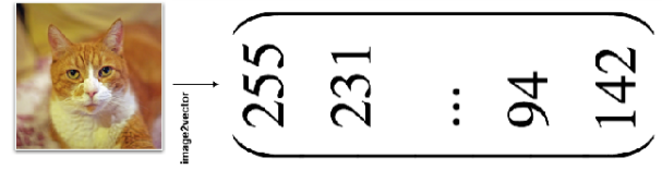
feature representation
The data needs to be converted into a numerical form that can be processed by the computer, and the image data needs to be converted into the representation of an RGB three-dimensional matrix.
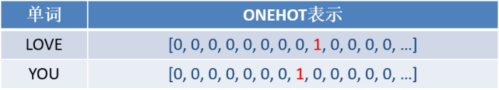
Character data can be represented by multidimensional arrays, such as Onehot one-hot encoding (represented by a single position of 1), word2vetor distributed representation, etc.;
Feature Derivation
Basic features have limited expression of sample information, and feature derivation can increase the nonlinear expression ability of features and improve the model effect. In addition, understanding the design features in the business can also increase the interpretability of the model. (For example, dividing weight by height is an important feature to express health conditions.) Feature derivation is to perform some processing (aggregation/conversion, etc.) on the meaning of existing basic features. Common methods are manual design and automatic feature derivation (Figure 4.15): ① Combined with the understanding of the business to do artificial derivative design: the way of aggregation refers to calculating the average value, count, maximum value, etc. after the field is aggregated. For example, the 12-month salary can be processed: the average monthly salary, the maximum salary, etc.; the conversion method refers to addition, subtraction, multiplication, and division between fields. For example, through 12 months of wages, it can be processed: the ratio and difference between wage income and expenditure of the current month, etc.;
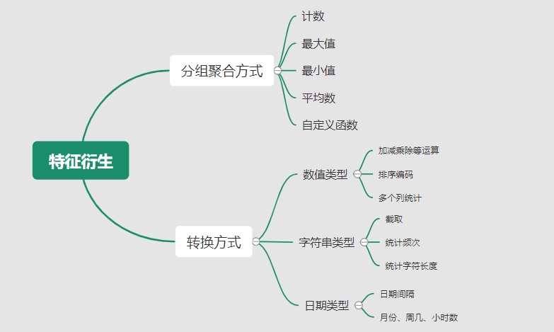
② Use automated feature derivative tools: such as Featuretools, etc., you can use aggregation (agg_primitives), conversion (trans_primitives) or custom methods to violently generate features;
feature selection
The goal of feature selection is to find the optimal feature subset, reduce the risk of over-fitting of the model and improve operating efficiency by screening out significant features and discarding redundant features. Feature selection methods are generally divided into three categories: ① Filtering method: Calculate the lack of features, divergence, correlation, information volume, stability and other types of indicators to evaluate and select each feature, commonly used such as missing rate, single value rate, Variance verification, pearson correlation coefficient, chi2 chi-square test, IV value, information gain and PSI and other methods. ② Packaging method: Iteratively trains the model by selecting part of the features each time, and selects the feature selection according to the model prediction effect score, such as sklearn's RFE recursive feature elimination. ③ Embedding method: Directly use some model training to understand the importance of features, and perform feature selection during model training. The weight coefficient of each feature is obtained through the model, and the feature is selected according to the weight coefficient from large to small. Commonly used such as logistic regression based on L1 regular term, XGBOOST feature importance selection feature.

feature dimensionality reduction
If the number of features after feature selection is still too large, in this case, there will often be problems with sparse data samples and difficult distance calculations (called the "curse of dimensionality"), which can be solved by feature dimensionality reduction. Commonly used dimensionality reduction methods are: principal component analysis (PCA) and so on.
3 Model training
Model training is the process of using established model methods to learn data experience. This process also needs to be combined with model evaluation to adjust the hyperparameters of the algorithm, and finally select a model with better performance.
3.1 Dataset division
Before training the model, the commonly used HoldOut verification method (in addition to leave-one-out method, k-fold cross-validation and other methods) divides the data set into training set and test set, and the training set can be further subdivided into training set and verification set to facilitate the evaluation of the performance of the model. ① Training set (training set): used to run the learning algorithm and train the model. ② The development set (development set) is used to adjust hyperparameters, select features, etc., to select a suitable model. ③ The test set (test set) is only used to evaluate the performance of the selected model, but will not change the learning algorithm or parameters accordingly. ###3.2 Model method selection Select the appropriate model method based on the current task and data conditions. The commonly used methods are shown in the figure below, the selection of scikit-learn model method. In addition, multiple models can be combined for model fusion.

3.3 Training process
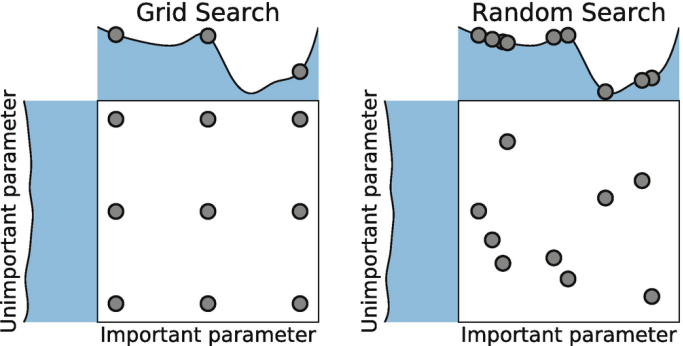
The training process of the model is to learn the data experience to obtain a better model and corresponding parameters (for example, the neural network finally learns a better weight value). The entire training process also needs to be controlled and optimized by adjusting hyperparameters (such as the number of neural network layers and the learning rate of gradient descent). Adjusting hyperparameters is an empirical process based on data sets, models, and details of the training process. It needs to be based on the understanding of the principles of the algorithm and experience, with the help of model evaluation in the validation set for parameter tuning. In addition, there is an automatic parameter tuning technology: grid Search, Random Search, Bayesian Optimization, etc.
4 Model evaluation
The direct purpose of machine learning is to learn (fit) a "good" model, not only to have a good learning and prediction ability for training data in the learning process, but also to have a good prediction ability for new data (general ability), so it is crucial to objectively evaluate model performance. Technically, the performance of the model is often evaluated based on the index performance of the training set and the test set.
4.1 Evaluation Indicators
Evaluate classification models
Commonly used evaluation criteria include precision rate P, recall rate R, and the harmonic average F1-score of the two, etc., and the value is calculated from the corresponding number of statistics of the confusion matrix:
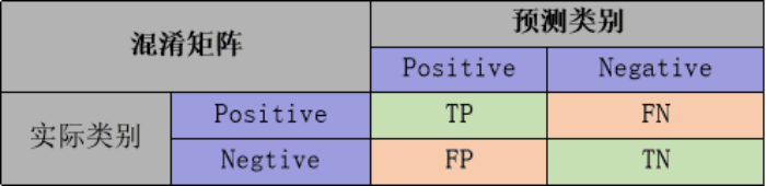
The precision rate refers to the ratio of the number of positive samples (TP) correctly classified by the classifier to the number of positive samples (TP+FP) predicted by the classifier; the recall rate refers to the number of positive samples correctly classified by the classifier. The number (TP) accounts for the proportion of all positive samples (TP+FN). F1-score is the harmonic average of precision P and recall R:

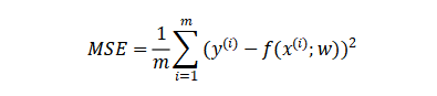
Evaluate regression models
Commonly used evaluation indicators are MSE mean square error and so on. Feedback is the fit between the predicted value and the actual value.
Evaluate the clustering model
It can be divided into two categories, one is to compare the clustering results with the results of a "reference model", which is called "external index" (external index): such as Rand index, FM index, etc. The other is to directly inspect the clustering results without using any reference model, which is called "internal index" (internal index): such as compactness, separation, etc.
4.2 Model evaluation and optimization
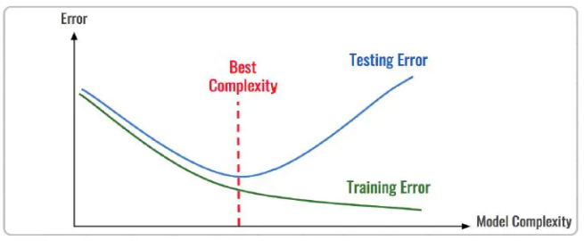
The data sample set used to train the machine learning model is called the training set, the error on the training data is called the training error, and the error on the test data is called the test error. ) or generalization error.
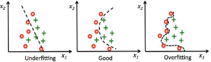
To describe the degree of model fitting (learning), underfitting, good fitting, and overfitting are commonly used. We can evaluate the degree of fitting of the model through training error and test error. From the perspective of the overall training process, the training error and test error are high when under-fitting, and decrease with the increase of training time and model complexity. After reaching a critical point of optimal fitting, the training error decreases and the test error increases, and at this time it enters the over-fitting region.
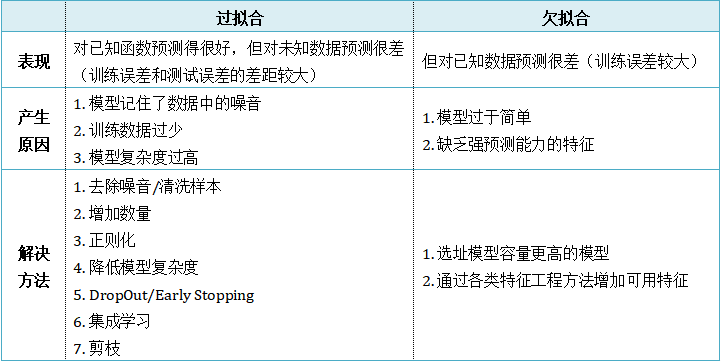
Underfitting means that the model structure is too simple compared to the data, so that the laws in the data cannot be learned. Overfitting means that the model only matches the training data set too much, so that it does not fit and predict new data well. Its essence is caused by the statistical noise learned by the more complex model from the training data. To analyze the model fitting effect and optimize the model, the commonly used methods are:
5 Model Decision
Decision-making application is the ultimate goal of machine learning. It analyzes and interprets the model prediction information and applies it to the actual work field. It should be noted that engineering is result-oriented, and the effect of the model running online directly determines the success or failure of the model, not only including its accuracy, error, etc., but also its running speed (time complexity), resource consumption ( Space complexity), comprehensive consideration of stability.
6 Machine Learning Project Combat (Data Mining)
6.1 Project Introduction
The experimental data of the project comes from the famous UCI machine learning database, which has a large amount of artificial intelligence data mining data. This example uses the version of the data set on sklearn: Breast Cancer Wisconsin DataSet (Wisconsin breast cancer data set), these data come from the clinical case reports of the University of Wisconsin Hospital in the United States. Oncology, the problem of supervised classification prediction. The modeling idea of the project is to analyze the breast cancer dataset data, feature engineering, construct a logistic regression model to learn the data, and predict whether the category of the sample is a benign tumor.
6.2 Code implementation
Import the relevant Python library, load the cancer dataset, view the data introduction, and convert it to DataFrame format.
import numpy as np
import pandas as pd
import matplotlib.pyplot as plt

from keras.models import Sequential
from keras.layers import Dense, Dropout
from keras.utils import plot_model
from sklearn import datasets
from sklearn.preprocessing import StandardScaler
from sklearn.model_selection import train_test_split
from sklearn.metrics import precision_score, recall_score, f1_score
dataset_cancer = datasets.load_breast_cancer() # 加载癌细胞数据集
print(dataset_cancer['DESCR'])
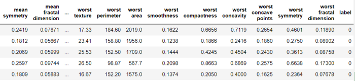
df = pd.DataFrame(dataset_cancer.data, columns=dataset_cancer.feature_names)
df['label'] = dataset_cancer.target
print(df.shape)
df.head()
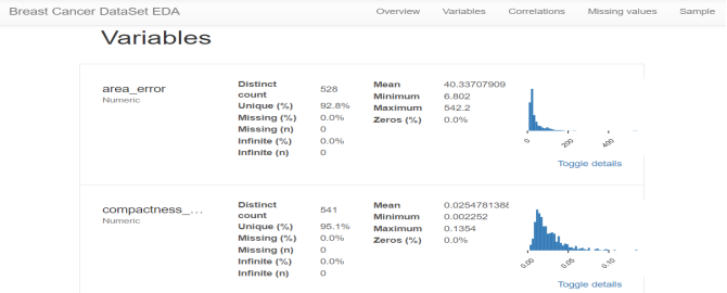
Exploratory data analysis EDA: Use the pandas_profiling library to analyze the data value, missing rate and correlation, etc.
import pandas_profiling

pandas_profiling.ProfileReport(df, title='Breast Cancer DataSet EDA')
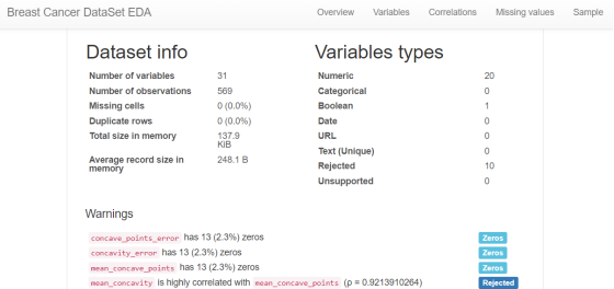
The main analysis and processing of feature engineering are:
● There is no obvious outlier or missing situation in the analysis feature, no need to deal with it;
● Derivative features such as mean/standard error exist, no need for feature derivation;
● Combining with correlation and other indicators for feature selection (filtering method);
● Normalize features to speed up the model learning process;
# 筛选相关性>0.99的特征清单列表及标签
drop_feas = ['label','worst_radius','mean_radius']

# 选择标签y及特征x
y = df.label
x = df.drop(drop_feas,axis=1)  # 删除相关性强特征及标签列

# holdout验证法: 按3:7划分测试集 训练集
x_train, x_test, y_train, y_test = train_test_split(x, y, test_size=0.3)

# 特征z-score 标准化
sc = StandardScaler()

x_train = sc.fit_transform(x_train)  # 注:训练集测试集要分别标准化,以免测试集信息泄露到模型训练
x_test = sc.transform(x_test)
Model training: use keras to build a logistic regression model, train the model, and observe the loss of the model training set and verification set
_dim = x_train.shape[1]   # 输入模型的特征数

# LR逻辑回归模型
model = Sequential()

model.add(Dense(1, input_dim=_dim, activation='sigmoid',bias_initializer='uniform'))  # 添加网络层,激活函数sigmoid

model.summary()

plot_model(model,show_shapes=True)
model.compile(optimizer='adam', loss='binary_crossentropy')  #模型编译:选择交叉熵损失函数及adam梯度下降法优化算法

model.fit(x, y, validation_split=0.3, epochs=200)   # 模型迭代训练: validation_split比例0.3, 迭代epochs200次

# 模型训练集及验证集的损失

plt.figure()

plt.plot(model.history.history['loss'],'b',label='Training loss')

plt.plot(model.history.history['val_loss'],'r',label='Validation val_loss')

plt.title('Traing and Validation loss')

plt.legend()
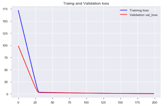
The generalization ability of the model is evaluated by the performance of the test set F1-score and other indicators. The f1-score of the final test set is 88%, which has a good model performance.

def model_metrics(model, x, y):
    """

    评估指标

    """
    yhat = model.predict(x).round()  # 模型预测yhat,预测阈值按默认0.5划分

    result = {


              'f1_score': f1_score(y, yhat),

              'precision':precision_score(y, yhat),

              'recall':recall_score(y, yhat)
             }

    return result

# 模型评估结果

print("TRAIN")

print(model_metrics(model, x_train, y_train))

print("TEST")

print(model_metrics(model, x_test, y_test))