Time Series Analysis - Based on R | Chapter 3 Properties of ARMA Model
Previous articles
Time series analysis - based on R | Chapter 1 exercise code
Time series analysis - based on R | Chapter 2 preprocessing exercise code of time series
-
It is known that a certain AR (1) AR(1)A R ( 1 ) model is:xt = 0.7 xt − 1 + ε t , ε t ∼ WN ( 0 , 1 ). x_t=0.7x_{t-1}+\varepsilon_t,\varepsilon_t \sim WN(0,1).xt=0.7x _t−1+et,et∼WN(0,1).求 E ( x t ) , V a r ( x t ) , ρ 2 E(x_t),Var(x_t),\rho_2 And ( xt),There is ( xt),r2and ϕ 22 . \phi_{22}.ϕ22.
E ( x t ) = ϕ 0 1 − ϕ 1 = 0 1 − 0.7 = 0 E\left(x_t\right)=\frac{\phi_{0}}{1-\phi_{1}}=\frac{0}{1-0.7}=0 E(xt)=1 − ϕ1ϕ0=1−0.70=0
V a r ( x t ) = 1 1 − ϕ 1 2 = 1 1 − 0. 7 2 = 1.96 Var(x_t)=\frac{1}{1-\phi_{1}^{2}}=\frac{1}{1-0.7^2}=1.96 There is ( xt)=1 − ϕ121=1−0.721=1.96
ρ 2 = ϕ 1 2 = 0.7 2 = 0.49 \rho_2=\phi_1^2=0.7^2=0.49r2=ϕ12=0.72=0.49
ϕ 22 = ∣ 1 ρ 1 ρ 1 ρ 2 ∣ ∣ 1 ρ 1 ρ 1 1 ∣ = 0.49 − 0. 7 2 1 − 0. 7 2 = 0 \phi_{22}=\frac{\left|\begin{array}{cc}1 & \rho_{1} \\\rho_{1} & \rho_{2}\end{array}\right|}{\left|\begin{array}{cc}1 & \rho_{1} \\\rho_{1} & 1\end{array}\right|}=\frac{0.49-0.7^{2}}{1-0.7^{2}}=0 ϕ22= 1r1r11 1r1r1r2 =1−0.720.49−0.72=0
-
It is known that a certain AR ( 2 ) \operatorname{AR}(2)AR ( 2 ) model:xt = ϕ 1 xt − 1 + ϕ 2 xt − 2 + ε t , ε t ∼ WN ( 0 , σ ε 2 ) x_t=\phi_1 x_{t-1}+\phi_2 x_{ t-2}+\varepsilon_t, \varepsilon_t \sim WN\left(0, \sigma_{\varepsilon}^2\right)xt=ϕ1xt−1+ϕ2xt−2+et,et∼WN(0,pe2) , andρ 1 = \rho_1=r1= 0.5 , ρ 2 = 0.3 0.5, \rho_2=0.3 0.5,r2=0.3 , 求ϕ 1 , ϕ 2 \phi_1, \phi_2ϕ1,ϕ2value.
A R ( 2 ) A R(2) A R ( 2 ) model:
{ ρ 1 = ϕ 1 1 − ϕ 2 ρ 2 = ϕ 1 ρ 1 + ϕ 2 ⇒ { 0.5 = ϕ 1 1 − ϕ 2 0.3 = 0.5 ϕ 1 + ϕ 2 ⇒ { ϕ 1 = 7 15 , ϕ 2 = 1 15 ϕ 2 = 1 15 \left\{\begin{array} { l } { \rho _ { 1 } = \frac { \phi _ { 1 } } { 1 - \phi _ { 2 } } } \\ { \rho _ { 2 } = \phi _ { 1 } \rho _ { 1 } + \phi _ { 2 } } \end{array} \Rightarrow \left\{\begin{array } { l } { 0 . 5 = \frac { \phi _ { 1 } } { 1 - \phi _ { 2 } } } \\ { 0 . 3 = 0. 5 \phi _ { 1 } + \phi _ { 2 } } \end{array} \Rightarrow \left\{\begin{array}{l} \phi_1=\frac{7}{15}, \phi_2=\ frac{1}{15} \\ \phi_2=\frac{1}{15} \end{array}\right.\right.\right.{ r1=1 − ϕ2ϕ1r2=ϕ1r1+ϕ2⇒{ 0.5=1 − ϕ2ϕ10.3=0.5 ϕ1+ϕ2⇒{ ϕ1=157,ϕ2=151ϕ2=151 -
It is known that a certain AR ( 2 ) \operatorname{AR}(2)The AR ( 2 ) model is:(1 − 0.5 B) (1 − 0.3 B) xt = ε t, ε t ∼ WN (0, 1) (1-0.5 B)(1-0.3 B) x_t=\varepsilon_t, \varepsilon_t \sim WN(0,1)(1−0.5B)(1−0.3 B ) xt=et,et∼WN(0,1), 求 E ( x t ) E\left(x_t\right) E(xt) ,Var ( xt ) , ρ k , ϕ kk \operatorname{Var}\left(x_t\right), \rho_k, \phi_{kk}Was(xt),rk,ϕkk, where k = 1, 2, 3 k=1,2,3k=1,2,3.
(1) ( 1 − 0.5 B ) ( 1 − 0.3 B ) x t = ε t ⇔ x t = 0.8 x t − 1 − 0.15 x t − 2 + ε t (1-0.5 B)(1-0.3 B) x_t=\varepsilon_t \Leftrightarrow x_t=0.8 x_{t-1}-0.15 x_{t-2}+\varepsilon_t (1−0.5B)(1−0.3 B ) xt=et⇔xt=0.8 xt−1−0.15xt−2+et
E ( xt ) = ϕ 0 1 − ϕ 1 − ϕ 2 = 0 E\left(x_t\right)=\frac{\phi_0}{1-\phi_1-\phi_2}=0E(xt)=1−ϕ1−ϕ2ϕ0=0
(2)
Var ( x t ) = 1 − ϕ 2 ( 1 + ϕ 2 ) ( 1 − ϕ 1 − ϕ 2 ) ( 1 + ϕ 1 − ϕ 2 ) = 1 + 0.15 ( 1 − 0.15 ) ( 1 − 0.8 + 0.15 ) ( 1 + 0.8 + 0.15 ) = 1.98 \begin{aligned} \operatorname{Var}\left(x_t\right) & =\frac{1-\phi_2}{\left(1+\phi_2\right)\left(1-\phi_1-\phi_2\right)\left(1+\phi_1-\phi_2\right)} \\ & =\frac{1+0.15}{(1-0.15)(1-0.8+0.15)(1+0.8+0.15)} \\ & =1.98 \end{aligned} Was(xt)=(1+ϕ2)(1−ϕ1−ϕ2)(1+ϕ1−ϕ2)1−ϕ2=(1−0.15)(1−0.8+0.15)(1+0.8+0.15)1+0.15=1.98
(3)
ρ 1 = ϕ 1 1 − ϕ 2 = 0.8 1 + 0.15 = 0.70 ρ 2 = ϕ 1 ρ 1 + ϕ 2 = 0.8 × 0.7 − 0.15 = 0.41 ρ 3 = ϕ 1 ρ 2 + ϕ 2 ρ 1 = 0.8 × 0.41 − 0.15 × 0.7 = 0.22 \begin{aligned} & \rho_1=\frac{\phi_1}{1-\phi_2}=\frac{0.8}{1+0.15}=0.70 \\ & \rho_2=\ phi_1 \rho_1+\phi_2=0.8 \times 0.7-0.15=0.41 \\ & \rho_3=\phi_1 \rho_2+\phi_2 \rho_1=0.8 \times 0.41-0.15 \times 0.7=0.22 \end{aligned}r1=1−ϕ2ϕ1=1+0.150.8=0.70r2=ϕ1r1+ϕ2=0.8×0.7−0.15=0.41r3=ϕ1r2+ϕ2r1=0.8×0.41−0.15×0.7=0.22
(4)
ϕ 11 = ρ 1 = 0.7 ϕ 22 = ϕ 2 = − 0.15 ϕ 33 = 0 \begin{aligned} \phi_{11} & =\rho_1=0.7 \\ \phi_{22} & =\phi_2= -0.15 \\ \phi_{33} & =0 \end{aligned}ϕ11ϕ22ϕ33=r1=0.7=ϕ2=−0.15=0 -
It is known that AR ( 2 ) \operatorname{AR}(2)The sequence of AR ( 2 ) is xt = xt − 1 + cxt − 2 + ε t x_t=x_{t-1}+c x_{t-2}+\varepsilon_txt=xt−1+cxt−2+et, where { ε t } \left\{\varepsilon_t\right\}{ et} is a white noise sequence. DetermineccThe value range of c is to ensure that{ xt } \left\{x_t\right\}{ xt} is a stationary sequence, and the sequenceρ k \rho_krkexpression.
(1) A R ( 2 ) A R(2) The stationary condition of the A R ( 2 ) model is
{ ∣ c ∣ < 1 c ± 1 < 1 ⇒ { − 1 < c < 1 c < 0 ⇒ − 1 < c < 0 \left\{\begin{array}{l}|c|<1 \\ c \pm 1<1\end{array} \Rightarrow\left\{\begin{array}{l}-1<c<1 \\ c<0\end{array} \Rightarrow-1<c<0\right.\right. { ∣c∣<1c±1<1⇒{ −1<c<1c<0⇒−1<c<0
(2) { ρ 1 = 1 1 − c , ρ k = ρ k − 1 + c ρ k − 2 , k ≥ 2 \left\{\begin{array}{l}\rho_{1}=\frac{ 1}{1-c}, \\\rho_{k}=\rho_{k-1}+c \rho_{k-2}, k \geq 2\end{array}\right.{ r1=1−c1,rk=rk−1+cρk−2,k≥2
-
Prove that for any constant ccc , AR (3) defined as follows\mathrm{AR}(3)The AR ( 3 ) sequence must be a non-stationary sequence:
xt = xt − 1 + cxt − 2 − cxt − 3 + ε t , ε t ∼ WN ( 0 , σ ε 2 ) x_t=x_{t-1}+c x_{ t-2}-c x_{t-3}+\varepsilon_t, \varepsilon_t \sim WN\left(0, \sigma_{\varepsilon}^2\right)xt=xt−1+cxt−2−cxt−3+et,et∼WN(0,pe2)
Proof:
The characteristic equation of this sequence is: λ 3 − λ 2 − c λ + c = 0 \lambda^{3}-\lambda^{2}-c \lambda+c=0l3−l2−c l+c=0 , solving this characteristic equation yields three characteristic roots:
λ 1 = 1 , λ 2 = c , λ 3 = − c \lambda_{1}=1, \quad \lambda_{2}=\sqrt{c}, \quad \lambda_{3}=-\sqrt{c} l1=1,l2=c,l3=−c
Regardless of ccNo matter what value c takes, this equation has a characteristic root on the unit circle, so the sequence must be a non-stationary sequence. Certification completed.
-
For AR ( 1 ) \mathrm{AR}(1)AR ( 1 ) model:xt = ϕ 1 xt − 1 + ε t , ε t ∼ WN ( 0 , σ ε 2 ) x_t=\phi_1 x_{t-1}+\varepsilon_t, \varepsilon_t \sim WN\left( 0, \sigma_{\varepsilon}^2\right)xt=ϕ1xt−1+et,et∼WN(0,pe2) , determine whether the following proposition is correct:
(1)γ 0 = ( 1 + ϕ 1 2 ) σ ε 2 \gamma_0=\left(1+\phi_1^2\right) \sigma_{\varepsilon}^2c0=(1+ϕ12)pe2
(2) E [ ( x t − μ ) ( x t − 1 − μ ) ] = − ϕ 1 E\left[\left(x_t-\mu\right)\left(x_{t-1}-\mu\right)\right]=-\phi_1 E[(xt−m )(xt−1−m ) ]=− ϕ1
(3) ρ k = ϕ 1 k \rho_k=\phi_1^krk=ϕ1k
(4) ϕ kk = ϕ 1 k \phi_{kk}=\phi_1^kϕkk=ϕ1k
(5) ρ k = ϕ 1 ρ k − 1 \rho_k=\phi_1\rho_{k-1}rk=ϕ1rk−1
Sure! Here are the answers and calculation processes for each statement:
(1) 错误。 γ 0 = σ ε 2 1 − ϕ 1 2 \gamma_0=\frac{\sigma_{\varepsilon}^2}{1-\phi_1^2} c0=1 − ϕ12pe2。
(2) 错误。 E [ ( x t − μ ) ( x t − 1 − μ ) ] = ϕ 1 γ 1 E\left[ \left(x_t-\mu\right)\left(x_{t-1}-\mu\right) \right]=\phi_1\gamma_1 E[(xt−m )(xt−1−m ) ]=ϕ1c1Let
E ( xt ) = E [ ϕ 1 xt − 1 + ε t ] = ϕ 1 E ( xt − 1 ) + E ( ε t ) = ϕ 1 E ( xt ) + 0 = 0 \begin{aligned } E(x_t) &= E[\phi_1x_{t-1}+\varepsilon_t] \\ &= \phi_1E(x_{t-1})+E(\varepsilon_t) \\ &= \phi_1E(x_t)+ 0 \\ &= 0 \end{aligned}And ( xt)=E [ ϕ1xt−1+et]=ϕ1And ( xt−1)+E ( et)=ϕ1And ( xt)+0=0
From this we can get μ = 0 \mu=0m=0も,Given:
E [ ( xt − μ ) ( xt − 1 − μ ) ] = E [ xtxt − 1 ] = E [ ( ϕ 1 xt − 1 + ε t ) xt − 1 ] = ϕ 1 E xt − 1 2 ] + E [ ε txt − 1 ] = ϕ 1 γ 0 \begin{aligned} E\left[\left(x_t-\mu\right)\left(x_{t-1}-\mu\ right)\right] &= E[x_tx_{t-1}] \\ &= E[(\phi_1x_{t-1}+\varepsilon_t)x_{t-1}] \\ &= \phi_1 E[x_ {t-1}^2] + E[\varepsilon_t x_{t-1}] \\ &= \phi_1 \gamma_0 \end{aligned}E[(xt−m )(xt−1−m ) ]=And [ xtxt−1]=E [( ϕ1xt−1+et)xt−1]=ϕ1And [ xt−12]+E [ etxt−1]=ϕ1c0
Therefore, the proposition is false.
(3) Correct. Since the AR(1) model has stationarity and finite second-order moment properties, when k > 0 k > 0k>When 0 , there isρ k = ϕ 1 k \rho_k=\phi_1^krk=ϕ1k
(4) Definition ϕ kk = { ϕ 1 , k = 1 0 , k ⩾ 2 \phi_{kk}=\begin{cases}\phi_1,&k=1\\ 0,&k\geqslant2\end{cases }ϕkk={ ϕ1,0,k=1k⩾2
(5) Correct. Since the AR(1) model has stationarity and finite second-order moment properties, when k > 0 k > 0k>When 0 , there isρ k = ϕ 1 ρ k − 1 \rho_k=\phi_1\rho_{k-1}rk=ϕ1rk−1。 -
It is known that a certain centralized MA (1) \mathrm{MA}(1)MA ( 1 ) model first-order autocorrelation coefficientρ 1 = 0.4 \rho_1=0.4r1=0.4 , find the expression of this model.
ρ 1 = − θ 1 1 + θ 1 2 = 0.4 ⇒ 0.4 θ 1 2 + θ 1 + 0.4 = 0 ⇒ θ 1 = − 2 or θ 1 = − 1 2 \rho_{ 1}=\frac{-\theta_{1}}{1+\theta_{1}^{2}}=0.4 \Rightarrow 0.4 \theta_{1}^{2}+\theta_{1}+0.4=0 \Rightarrow \theta_{1}=-2 \text { or} \theta_{1}=-\frac{1}{2}r1=1+i12− i1=0.4⇒0.4 i12+i1+0.4=0⇒i1=− 2 or θ 1=−21So the model has two possible expressions: xt = ε t + 1 2 ε t − 1 x_{t}=\varepsilon_{t}+\frac{1}{2} \varepsilon_{t-1}xt=et+21et−1和xt = ε t + 2 ε t − 1 x_{t}=\varepsilon_{t}+2 \varepsilon_{t-1}xt=et+2 et−1 。
-
Determine the constant CCThe value of C is to ensure that the following expression isMA (2) \mathrm{MA}(2)MA ( 2 ) model:
xt = 10 + 0.5 xt − 1 + ε t − 0.8 ε t − 2 + C ε t − 3 x_t=10+0.5 x_{t-1}+\varepsilon_t-0.8 \varepsilon_{t-2}+C \varepsilon_ {t-3}xt=10+0.5x _t−1+et−0.8 et−2+C εt−3
将xt = 10 + 0.5 xt − 1 + ε t − 0.8 ε t − 2 + C ε t − 3 x_{t}=10+0.5 x_{t-1}+\varepsilon_{t}-0.8 \varepsilon_{ t-2}+C \varepsilon_{t-3}xt=10+0.5x _t−1+et−0.8 et−2+C εt−3The equivalent expression is
xt − 10 = 1 − 0.8 B 2 + c B 3 1 − 0.5 B ε t = ( 1 + a B + b B 2 ) ε t x_{t}-10=\frac{1-0.8 B ^{2}+c B^{3}}{1-0.5 B} \varepsilon_{t}=\left(1+a B+b B^{2}\right) \varepsilon_{t}xt−10=1−0.5B1−0.8B2+cB3et=(1+aB+bB2)et
Rules
1 − 0.8 B 2 + c B 3 = ( 1 + a B + b B 2 ) ( 1 − 0.5 B ) = 1 + ( a − 0.5 ) B + ( b − 0.5 a ) B 2 − 0.5 b B 3 \begin{aligned} 1-0.8 B^{2}+c B^{3} & =\left(1+a B+b B^{2}\right)(1-0.5 B) \\ & =1+(a-0.5) B+(b-0.5 a) B^{2}-0.5 b B^{3} \end{aligned} 1−0.8B2+cB3=(1+aB+bB2)(1−0.5B)=1+(a−0.5)B+(b−0.5a)B2−0.5 bB _3
According to the undetermined coefficient method:
− 0.8 = a − 0.5 ⇒ a = − 0.3 0 = − 0.5 b ⇒ b = 0 c = b − 0.5 a ⇒ c = 0.15 \begin{aligned} -0.8 & =a-0.5 \Rightarrow a=-0.3 \\ 0 & =-0.5 b \Rightarrow b=0 \\ c & =b-0.5 a \Rightarrow c=0.15 \end{aligned} −0.80c=a−0.5⇒a=−0.3=−0.5b⇒b=0=b−0.5 a⇒c=0.15
-
Known MA (2) \mathrm{MA}(2)MA ( 2 ) model:xt = ε t − 0.7 ε t − 1 + 0.4 ε t − 2 , ε t ∼ WN ( 0 , σ ε 2 ) x_t=\varepsilon_t-0.7 \varepsilon_{t-1}+0.4 \varepsilon_{t-2}, \varepsilon_t \sim WN\left(0, \sigma_{\varepsilon}^2\right)xt=et−0.7εt−1+0.4εt−2,εt∼WN(0,σε2). 求 E ( x t ) , Var ( x t ) E\left(x_t\right), \operatorname{Var}\left(x_t\right) E(xt),Var(xt), 及 ρ k ( k ⩾ 1 ) \rho_k(k \geqslant 1) ρk(k⩾1).
(1) E ( x t ) = 0 E\left(x_{t}\right)=0 E(xt)=0
(2) Var ( x t ) = 1 + 0. 7 2 + 0. 4 2 = 1.65 \operatorname{Var}\left(x_{t}\right)=1+0.7^{2}+0.4^{2}=1.65 Var(xt)=1+0.72+0.42=1.65
(3) ρ 1 = − 0.7 − 0.7 × 0.4 1.65 = − 0.59 , ρ 2 = 0.4 1.65 = 0.24 , ρ k = 0 , k ≥ 3 \rho_{1}=\frac{-0.7-0.7 \times 0.4} {1.65}=-0.59, \quad \rho_{2}=\frac{0.4}{1.65}=0.24, \quad \rho_{k}=0, k \geq 3r1=1.65−0.7−0.7×0.4=−0.59,r2=1.650.4=0.24,rk=0,k≥3
-
prove:
(1) For any constant ccc , the infinite-order MA sequence defined as follows must be a non-stationary sequence:
xt = ε t + c ( ε t − 1 + ε t − 2 + ⋯ ) , ε t ∼ WN ( 0 , σ ε 2 ) x_{t}= \varepsilon_{t}+c\left(\varepsilon_{t-1}+\varepsilon_{t-2}+\cdots\right), \quad \varepsilon_{t} \sim WN\left(0, \sigma_{ \varepsilon}^{2}\right)xt=et+c( et−1+et−2+⋯),et∼WN(0,pe2)Proof: Because for any constant C, we have
Var ( xt ) = lim k → ∞ ( 1 + k C 2 ) σ ε 2 = ∞ \operatorname{Var}\left(x_{t}\right)=\lim_{k\rightarrow\infty}\ left ( 1 + k C ^ { 2 } \ right ) \ sigma_ { \ productpsilon } ^ { 2 } = \ inftyWas(xt)=k→∞lim(1+kC2)pe2=∞
Therefore, this series is a non-stationary series.
(2) { x t } \left\{x_{t}\right\} { xtThe first-order difference sequence of } must be a stationary sequence, and find { yt } \left\{y_{t}\right\}{ yt} Autocorrelation coefficient expression:
yt = xt − xt − 1 y_{t}=x_{t}-x_{t-1}yt=xt−xt−1yt = xt − xt − 1 = ε t + ( C − 1 ) ε t − 1 y_{t}=x_{t}-x_{t-1}=\varepsilon_{t}+(C-1) \varepsilon_ {t-1}yt=xt−xt−1=et+(C−1 ) et−1, then the sequence { yt } \left\{y_{t}\right\}{ yt} Satisfy the following conditions:
The mean and variance are constants,
E ( yt ) = 0 , Var ( yt ) = [ 1 + ( C − 1 ) 2 ] σ ε 2 E\left(y_{t}\right)=0, \operatorname{Var}\left(y_{ t}\right)=\left[1+(C-1)^{2}\right] \sigma_{\varepsilon}^{2}E(yt)=0,Was(yt)=[1+(C−1)2]pe2
The autocorrelation coefficient is only related to the length of the time interval and has nothing to do with the starting time
ρ 1 = C − 1 1 + ( C − 1 ) 2 , ρ k = 0 , k ≥ 2 \rho_{1}=\frac{C-1}{1+(C-1)^{2}}, \rho_{k}=0, k \geqr1=1+(C−1)2C−1,rk=0,k≥2
Therefore, the difference sequence is a stationary sequence.
-
Test the stationarity and reversibility of the following model, where { ε t } \left\{\varepsilon_{t}\right\}{ et} is a white noise sequence:
(1)xt = 0.5 xt − 1 + 1.2 xt − 2 + ε t x_{t}=0.5 x_{t-1}+1.2 x_{t-2}+\varepsilon_{t}xt=0.5x _t−1+1.2 xt−2+et
Test stationarity: The characteristic equation of this model is 1 − 0.5 z − 1.2 z 2 = 0 1-0.5z-1.2z^2=01−0.5 z−1.2 z2=0 , the solution is to obtain the characteristic roots asz 1 = 1.0517, z 2 = − 0.4784 z_1=1.0517,\,z_2=-0.4784z1=1.0517,z2=− 0.4784 . Since the modulus of one of the eigenvalues is greater than 1, the model is not stationary.
(2) xt = 1.1 xt − 1 − 0.3 xt − 2 + ε t x_{t}=1.1 x_{t-1}-0.3 x_{t-2}+\varepsilon_{t}xt=1.1xt−1−0.3x _t−2+et
Test stationarity: The characteristic equation of this model is 1 − 1.1 z + 0.3 z 2 = 0 1-1.1z+0.3z^2=01−1.1 z+0.3 z2=0 , the characteristic roots arez 1 = 0.3667, z 2 = 1.3667 z_1=0.3667, z_2=1.3667z1=0.3667,z2=1.3667 . Since∣ z 2 ∣ > 1 |z_2|>1∣z2∣>1 , so the model is not stationary.
(3) xt = ε t − 0.9 ε t − 1 + 0.3 ε t − 2 x_{t}=\varepsilon_{t}-0.9 \varepsilon_{t-1}+0.3 \varepsilon_{t-2}xt=et−0.9 et−1+0.3 et−2
Test stationarity: The characteristic equation of this model is 1 + 0.9 z − 0.3 z 2 = 0 1+0.9z-0.3z^2=01+0.9 z−0.3 z2=0 , the characteristic roots arez 1 = 0.5, z 2 = − 0.6 z_1=0.5,\,z_2=-0.6z1=0.5,z2=− 0.6 . Since the modulus length of all eigenroots is less than 1, the model is stationary. Testing reversibility: this model is consistent with ARMA(2, 2) (2,2)(2,2 ) The model is the same and therefore also reversible.
(4) xt = ε t + 1.3 ε t − 1 − 0.4 ε t − 2 x_{t}=\varepsilon_{t}+1.3 \varepsilon_{t-1}-0.4 \varepsilon_{t-2}xt=et+1.3 et−1−0.4 et−2
Test stationarity: The characteristic equation of this model is 1 − 1.3 z + 0.4 z 2 = 0 1-1.3z+0.4z^2=01−1.3z _+0.4z2=0 , the solution is to obtain the characteristic roots asz 1 = 1.465, z 2 = 0.272 z_1=1.465,\,z_2=0.272z1=1.465,z2=0.272 . The modulus of one of the eigenvalues is greater than 1, so the model is not stationary. Testing reversibility: this model is consistent with ARMA(2, 2) (2,2)(2,2 ) The models are the same and therefore irreversible.
(5) xt = 0.7 xt − 1 + ε t − 0.6 ε t − 1 x_{t}=0.7 x_{t-1}+\varepsilon_{t}-0.6 \varepsilon_{t-1}xt=0.7x _t−1+et−0.6 et−1
Test stationarity: The characteristic equation of this model is 1 − 0.7 z + 0.6 z 2 = 0 1-0.7z+0.6z^2=01−0.7 z+0.6 z2=0 , the characteristic roots arez 1 = 0.5, z 2 = 1 z_1=0.5,\,z_2=1z1=0.5,z2=1 . The modulus length of one of the characteristic roots is equal to 1, so the reversibility needs to be further tested. Testing reversibility: this model is consistent with ARMA( 1 , 1 ) (1,1)(1,1 ) The models are the same and therefore reversible.
(6) xt = − 0.8 xt − 1 + 0.5 xt − 2 + ε t − 1.1 ε t − 1 x_{t}=-0.8 x_{t-1}+0.5 x_{t-2}+\varepsilon_{ t}-1.1 \varepsilon_{t-1}xt=− 0.8 xt−1+0.5x _t−2+et−1.1 et−1
Test stationarity: The characteristic equation of this model is 1 + 0.8 z − 0.5 z 2 − 1.1 z − 1 = 0 1+0.8z-0.5z^2-1.1z^{-1}=01+0.8z _−0.5 z2−1.1 z−1=0,解得分内根的z 1 = 1.0501 , z 2 = 0.9804 ± 0.1083 i , z 3 = 0.9452 ± 0.2306 i , z 4 = 0.7889 ± 0.5491 i , z 5 = − 0.9258 ± 0.3732 i , z 6 = − 0.967 9 ± 0.2607 i , z 7 = − 0.9720 ± 0.2341 i , z 8 = − 0.9880 ± 0.1402 i , z 9 = − 0.9893 ± 0.1303 i , z 10 = − 1.0000 z_1=1.0501,\,z_2=0.9804\pm0.10 83i, \,z_3=0.9452\pm0.2306i,\,z_4=0.7889\pm0.5491i,\,z_5=-0.9258\pm0.3732i,\,z_6=-0.9679\pm0.2607i,\,z_7=-0.9720\pm0 .2341i,\,z_8=-0.9880\pm0.1402i,\,z_9=-0.9893\pm0.1303i,\,z_{10}=-1.0000z1=1.0501,z2=0.9804±0.1083i,z3=0.9452±0.2306i , _z4=0.7889±0.5491i,z5=−0.9258±0.3732i , _z6=−0.9679±0.2607i , _z7=−0.9720±0.2341 i ,z8=−0.9880±0.1402i,z9=−0.9893±0.1303i , _z10=− 1.0000 . One of the characteristic roots has a modulus greater than 1, so the model is not stationary. Test reversibility: Because the characteristic equation of this model contains an inversion operatorz − 1 z^{-1}z− 1 , so the model is not reversible.
To sum up, (1) is not stationary; (2) is not stationary; (3) is stationary and reversible; (4) is not stationary and irreversible; (5) is stationary and reversible; (6) is not Smooth and irreversible. -
It is known that ARMA ( 1 , 1 ) \operatorname{ARMA}(1,1)ARMA(1,1 ) The model is:xt = 0.6 xt − 1 + ε t − 0.3 ε t − 1 x_{t}=0.6 x_{t-1}+\varepsilon_{t}-0.3 \varepsilon_{t-1}xt=0.6x _t−1+et−0.3 et−1, determine the Green function of the model so that the model can be equivalently expressed as infinite MA \mathrm{MA}MA order model form.
The Green function of this model is:
G 0 = 1 G_{0}=1G0=1
G 1 = ϕ 1 G 0 − θ 1 = 0.6 − 0.3 = 0.3 G_{1}=\phi_{1} G_{0}-\theta_{1}=0.6-0.3=0.3G1=ϕ1G0−i1=0.6−0.3=0.3
G k = ϕ 1 G k − 1 = ϕ 1 k − 1 G 1 = 0.3 × 0. 6 k − 1 , k ≥ 2 G_{k}=\phi_{1} G_{k-1}=\phi_{1}^{k-1} G_{1}=0.3 \times 0.6^{k-1}, k \geq 2 Gk=ϕ1Gk−1=ϕ1k−1G1=0.3×0.6k−1,k≥2
So the model can be equivalently expressed as: xt = ε t + ∑ k = 0 ∞ 0.3 × 0. 6 k ε t − k − 1 x_{t}=\varepsilon_{t}+\sum_{k=0}^ {\infty} 0.3 \times 0.6^{k} \varepsilon_{tk-1}xt=et+∑k=0∞0.3×0.6k εt−k−1
-
某WEAPON ( 2 , 2 ) \operatorname{WEAPON}(2,2)ARMA(2,2 ) Definition:Φ ( B ) xt = 3 + Θ ( B ) ε ı \Phi(B) x_{t}=3+\Theta(B) \varepsilon_{\imath};Φ ( B ) xt=3+Θ ( B ) e, 求 E ( x t ) E\left(x_{t}\right) E(xt) . Among them,ε t ∼ WN ( 0 , σ ε 2 ) \varepsilon_{t} \sim WN\left(0, \sigma_{\varepsilon}^{2}\right)et∼WN(0,pe2) ,Φ ( B ) = ( 1 − 0.5 B ) 2 . \Phi(B)=(1-0.5 B)^{2}.Φ ( B )=(1−0.5B)2 .
Θ ( B ) = ( 1 − 0.5 B ) 2 ⇒ ϕ 1 = 0.5 , ϕ 2 = − 0.25 E ( xt ) = ϕ 0 1 − ϕ 1 − ϕ 2 = 3 1 − 0.5 + 0.25 = 4 \begin{aligned } & \Theta(B)=(1-0.5 B)^{2} \Rightarrow \phi_{1}=0.5, \quad \phi_{2}=-0.25 \\ & E\left(x_{t}\ right)=\frac{\phi_{0}}{1-\phi_{1}-\phi_{2}}=\frac{3}{1-0.5+0.25}=4 \end{aligned}Θ ( B )=(1−0.5B)2⇒ϕ1=0.5,ϕ2=−0.25E(xt)=1−ϕ1−ϕ2ϕ0=1−0.5+0.253=4 -
Prove ARMA ( 1 , 1 ) \operatorname{ARMA}(1,1)ARMA(1,1 ) seqxt= 0.5 xt − 1 + ε t − 0.25 ε t − 1 , ε t ∼ WN ( 0 , σ ε 2 ) x_{t}=0.5 x_{t-1}+\varepsilon_{t}-0.25 \varepsilon_{t-1}, \varepsilon_{t} \sim WN\left(0, \sigma_{\varepsilon}^{2}\right)xt=0.5x _t−1+et−0.25 et−1,et∼WN(0,pe2) ’s autocorrelation coefficient is:
ρ k = { 1 , k = 0 0.27 , k = 1 0.5 ρ k − 1 , k ⩾ 2 \rho_{k}= \begin{cases}1, & k=0 \\ 0.27, & k=1 \\ 0.5 \rho_{k-1}, & k \geqslant 2\end{cases}rk=⎩ ⎨ ⎧1,0.27,0.5 pk−1,k=0k=1k⩾2
Denominator 1 = 1 2 , θ 1 = 1 4 \phi_{1}=\frac{1}{2}, \theta_{1}=\frac{1}{4}ϕ1=21,i1=41, according to ARMA ( 1 , 1 ) ARMA(1,1)ARMA(1,1 ) The recursive formula of the model Green function is:
G 0 = 1 G_{0}=1G0=1 ,
G 1 = ϕ 1 G 0 − θ 1 = 0.5 − 0.25 = ϕ 1 2 G_{1}=\phi_{1} G_{0}-\theta_{1}=0.5-0.25=\phi_{1} ^{2}G1=ϕ1G0−i1=0.5−0.25=ϕ12
G k = ϕ 1 G k − 1 = ϕ 1 k − 1 G 1 = ϕ 1 k + 1 , k ≥ 2 G_{k}=\phi_{1} G_{k-1}=\phi_{1}^ {k-1} G_{1}=\phi_{1}^{k+1}, k \geq 2Gk=ϕ1Gk−1=ϕ1k−1G1=ϕ1k+1,k≥2
ρ 0 = 1 \rho_{0}=1 r0=1
ρ 1 = ∑ j = 0 ∞ G j G j + 1 ∑ j = 0 ∞ G j 2 = ϕ 1 2 + ∑ j = 1 ∞ ϕ 1 2 j + 3 1 + ∑ j = 1 ∞ ϕ 1 2 ( j + 1 ) = ϕ 1 2 + ϕ 1 5 1 − ϕ 1 2 1 + ϕ 1 4 1 − ϕ 1 2 = ϕ 1 2 − ϕ 1 4 + ϕ 1 5 1 − ϕ 1 2 + ϕ 1 4 = 7 26 = 0.27 ρ k = ∑ j = 0 ∞ G j G j + k ∑ j = 0 ∞ G j 2 = ∑ j = 0 ∞ G j ( ϕ 1 G j + k − 1 ) ∑ j = 0 ∞ G j 2 = ϕ 1 ∑ j = 0 ∞ G j G j + k − 1 ∑ j = 0 ∞ G j 2 = ϕ 1 ρ k − 1 , k ≥ 2 \begin{aligned} & \rho_{1}=\frac{ \sum_{j=0}^{\infty} G_{j} G_{j+1}}{\sum_{j=0}^{\infty} G_{j}^{2}}=\frac{\ phi_{1}^{2}+\sum_{j=1}^{\infty} \phi_{1}^{2 j+3}}{1+\sum_{j=1}^{\infty} \ phi_{1}^{2(j+1)}}=\frac{\phi_{1}^{2}+\frac{\phi_{1}^{5}}{1-\phi_{1}^ {2}}}{1+\frac{\phi_{1}^{4}}{1-\phi_{1}^{2}}}=\frac{\phi_{1}^{2}}\ phi_{1}^{4}+\phi_{1}^{5}}{1-\phi_{1}^{2}+\phi_{1}^{4}}=\frac{7}{26 }=0.27 \\ & \rho_{k}=\frac{\sum_{j=0}^{\infty} G_{j} G_{j+k}}{\sum_{j=0}^{\infty} G_{j}^{2}}=\frac{\sum_{j=0}^{\infty} G_{j}\left(\phi_{1} G_{j+k-1}\right)}{\sum_{j=0}^{\infty} G_{j}^{2}}=\phi_{1} \frac{\sum_{j=0}^{\infty} G_{j} G_{j+k-1}}{\sum_{j=0}^{\infty} G_{j}^{2}}=\phi_{1} \rho_{k-1}, k \geq 2 \end{aligned}r1=∑j=0∞Gj2∑j=0∞GjGj+1=1+∑j=1∞ϕ12(j+1)ϕ12+∑j=1∞ϕ12 j + 3=1+1 − ϕ12ϕ14ϕ12+1 − ϕ12ϕ15=1−ϕ12+ϕ14ϕ12−ϕ14+ϕ15=267=0.27rk=∑j=0∞Gj2∑j=0∞GjGj+k=∑j=0∞Gj2∑j=0∞Gj( ϕ1Gj+k−1)=ϕ1∑j=0∞Gj2∑j=0∞GjGj+k−1=ϕ1rk−1,k≥2
Certification completed.
- For stationary time series, which of the following equations must be true?
(1) σ ε 2 = E ( ε 1 2 ) \sigma_{\varepsilon}^{2}=E\left(\varepsilon_{1}^{2}\right)pe2=E( e12)
(2) Cov ( y t , y t + k ) = Cov ( y t , y t − k ) \operatorname{Cov}\left(y_{t}, y_{t+k}\right)=\operatorname{Cov}\left(y_{t}, y_{t-k}\right) Those(yt,yt+k)=Those(yt,yt−k)
(3) ρ k = ρ − k \rho_{k}=\rho_{-k} rk=r−k
(4) y ^ t ( k + 1 ) = y ^ t + 1 ( k ) \widehat{y}_{t}(k+1)=\widehat{y}_{t+1}(k) y t(k+1)=y t+1(k).
(1) Established
(2) Established
(3) Established
(4) Established
- The annual firearm-related homicide death rate (per 100,000 people) in Australia from 1915 to 2004 is shown in the table.
(1) If the series is judged to be stationary, please determine which model in ARMA the stationary series has.
(2) If the sequence is judged to be non-stationary, please examine the stationarity and correlation characteristics of the sequence after first-order difference.
年	死亡率
1915	0.5215052
1916	0.4248284
1917	0.4250311
1918	0.4771938
1919	0.8280212
1920	0.6156186
1921	0.366627
1922	0.4308883
1923	0.2810287
1924	0.4646245
1925	0.2693951
1926	0.5779049
1927	0.5661151
1928	0.5077584
1929	0.7507175
1930	0.6808395
1931	0.7661091
1932	0.4561473
1933	0.4977496
1934	0.4193273
1935	0.6095514
1936	0.457337
1937	0.5705478
1938	0.3478996
1939	0.3874993
1940	0.5824285
1941	0.2391033
1942	0.2367445
1943	0.2626158
1944	0.4240934
1945	0.365275
1946	0.3750758
1947	0.4090056
1948	0.3891676
1949	0.240261
1950	0.1589496
1951	0.4393373
1952	0.5094681
1953	0.3743465
1954	0.4339828
1955	0.4130557
1956	0.3288928
1957	0.5186648
1958	0.5486504
1959	0.5469111
1960	0.4963494
1961	0.5308929
1962	0.5957761
1963	0.5570584
1964	0.5731325
1965	0.5005416
1966	0.5431269
1967	0.5593657
1968	0.6911693
1969	0.4403485
1970	0.5676662
1971	0.5969114
1972	0.4735537
1973	0.5923935
1974	0.5975556
1975	0.6334127
1976	0.6057115
1977	0.7046107
1978	0.4805263
1979	0.702686
1980	0.7009017
1981	0.6030854
1982	0.6980919
1983	0.597656
1984	0.8023421
1985	0.6017109
1986	0.5993127
1987	0.6025625
1988	0.7016625
1989	0.4995714
1990	0.4980918
1991	0.497569
1992	0.600183
1993	0.3339542
1994	0.274437
1995	0.3209428
1996	0.5406671
1997	0.4050209
1998	0.2885961
1999	0.3275942
2000	0.3132606
2001	0.2575562
2002	0.2138386
2003	0.1861856
2004	0.1592713
1. Convert data into time series variables and visualize them:
data <- read.table('./时间序列分析——基于R(第2版)习题数据/习题3.16数据.txt', header = TRUE, sep = "\t")
#将年份转换为时间序列类型
death <- ts(data$死亡率, start = c(1915), end = c(2004), frequency = 1)
#可视化
plot(death, type = "l", main = "1915-2004年澳大利亚枪支凶杀案死亡率",
     xlab = "年份", ylab = "死亡率")

2. Perform a stationarity test on the time series:
library(tseries)
## Registered S3 method overwritten by 'quantmod':
##   method            from
##   as.zoo.data.frame zoo
#进行ADF检验
adf.test(death)
##
##  Augmented Dickey-Fuller Test
##
## data:  death
## Dickey-Fuller = -1.2491, Lag order = 4, p-value = 0.8853
## alternative hypothesis: stationary
#进行KPSS检验
kpss.test(death)
## Warning in kpss.test(death): p-value greater than printed p-value
##
##  KPSS Test for Level Stationarity
##
## data:  death
## KPSS Level = 0.19826, Truncation lag parameter = 3, p-value = 0.1
Conclusion:
The p-value of the ADF test is greater than 0.05, and the null hypothesis cannot be rejected, that is, the sequence is not stationary; the
p-value of the KPSS test is less than 0.05, and the null hypothesis is rejected, that is, the sequence is not stationary.
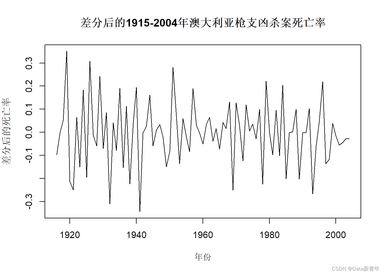
3. Perform the first-order difference operation and perform the stationarity test again:
diff_ts <- diff(death)
#可视化
plot(diff_ts, type = "l", main = "差分后的1915-2004年澳大利亚枪支凶杀案死亡率",
     xlab = "年份", ylab = "差分后的死亡率")
#进行ADF检验
adf.test(diff_ts)
## Warning in adf.test(diff_ts): p-value smaller than printed p-value
##
##  Augmented Dickey-Fuller Test
##
## data:  diff_ts
## Dickey-Fuller = -5.1026, Lag order = 4, p-value = 0.01
## alternative hypothesis: stationary
#进行KPSS检验
kpss.test(diff_ts)
## Warning in kpss.test(diff_ts): p-value greater than printed p-value
##
##  KPSS Test for Level Stationarity
##
## data:  diff_ts
## KPSS Level = 0.099305, Truncation lag parameter = 3, p-value = 0.1
Conclusion:
The sequence is significantly stationary after the first difference;
the p value of the KPSS test is greater than 0.05, and the null hypothesis cannot be rejected, that is, the sequence tends to be stationary under the first difference.
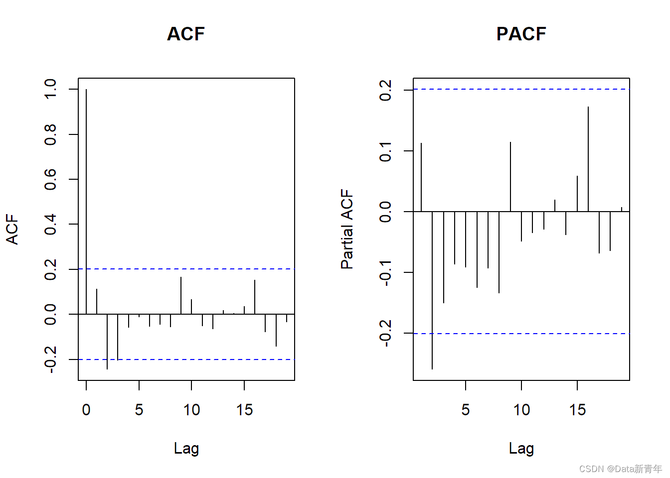
4. Perform ACF and PACF analysis on the first-differenced sequence to determine the ARMA model:
#ACF和PACF
par(mfrow = c(1,2))
acf(diff_ts, main = "ACF")
pacf(diff_ts, main = "PACF")
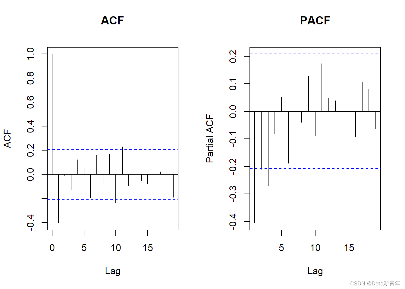
Conclusion:
ACF shows that the sequence has obvious adjacent lag autocorrelation, and PACF shows that the sequence has truncated autoregressive (AR) characteristics.
Therefore, one can choose the ARMA(p,0) model, where p takes a value of 2 or 3.
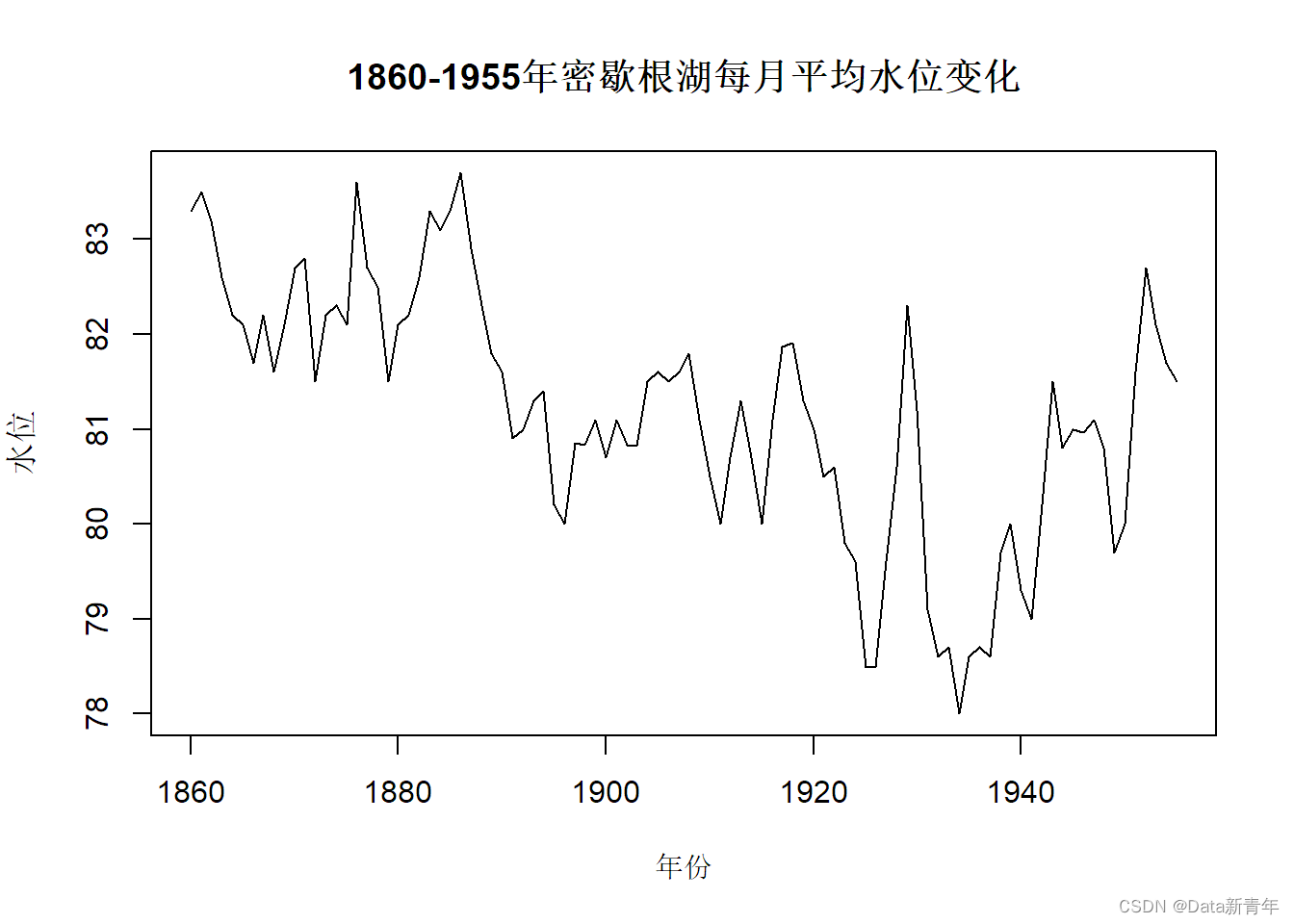
- The sequence of maximum monthly average water levels in Lake Michigan from 1860 to 1955 is shown in the table below.
(1) If the series is judged to be stationary, please determine which model in ARMA the stationary series has.
(2) If the sequence is judged to be non-stationary, please examine the stationarity and correlation characteristics of the sequence after first-order difference.
年	水位
1860	83.3
1861	83.5
1862	83.2
1863	82.6
1864	82.2
1865	82.1
1866	81.7
1867	82.2
1868	81.6
1869	82.1
1870	82.7
1871	82.8
1872	81.5
1873	82.2
1874	82.3
1875	82.1
1876	83.6
1877	82.7
1878	82.5
1879	81.5
1880	82.1
1881	82.2
1882	82.6
1883	83.3
1884	83.1
1885	83.3
1886	83.7
1887	82.9
1888	82.3
1889	81.8
1890	81.6
1891	80.9
1892	81
1893	81.3
1894	81.4
1895	80.2
1896	80
1897	80.85
1898	80.83
1899	81.1
1900	80.7
1901	81.1
1902	80.83
1903	80.82
1904	81.5
1905	81.6
1906	81.5
1907	81.6
1908	81.8
1909	81.1
1910	80.5
1911	80
1912	80.7
1913	81.3
1914	80.7
1915	80
1916	81.1
1917	81.87
1918	81.91
1919	81.3
1920	81
1921	80.5
1922	80.6
1923	79.8
1924	79.6
1925	78.49
1926	78.49
1927	79.6
1928	80.6
1929	82.3
1930	81.2
1931	79.1
1932	78.6
1933	78.7
1934	78
1935	78.6
1936	78.7
1937	78.6
1938	79.7
1939	80
1940	79.3
1941	79
1942	80.2
1943	81.5
1944	80.8
1945	81
1946	80.96
1947	81.1
1948	80.8
1949	79.7
1950	80
1951	81.6
1952	82.7
1953	82.1
1954	81.7
1955	81.5
1. Convert data into time series variables and visualize them:
data <- read.table('./时间序列分析——基于R(第2版)习题数据/习题3.17数据.txt', header = TRUE, sep = "\t")
#将年份转换为时间序列类型
level <- ts(data$水位, start = c(1860), end = c(1955), frequency = 1)
#可视化
plot(level, type = "l", main = "1860-1955年密歇根湖每月平均水位变化",
     xlab = "年份", ylab = "水位")
2. Perform a stationarity test on the time series:
library(tseries)
#进行ADF检验
adf.test(level)
##
##  Augmented Dickey-Fuller Test
##
## data:  level
## Dickey-Fuller = -2.3833, Lag order = 4, p-value = 0.4181
## alternative hypothesis: stationary
#进行KPSS检验
kpss.test(level)
## Warning in kpss.test(level): p-value smaller than printed p-value
##
##  KPSS Test for Level Stationarity
##
## data:  level
## KPSS Level = 1.3798, Truncation lag parameter = 3, p-value = 0.01
Conclusion:
The p-value of the ADF test is greater than 0.05, and the null hypothesis cannot be rejected, that is, the sequence is not stationary; the
p-value of the KPSS test is less than 0.05, and the null hypothesis is rejected, that is, the sequence is not stationary.
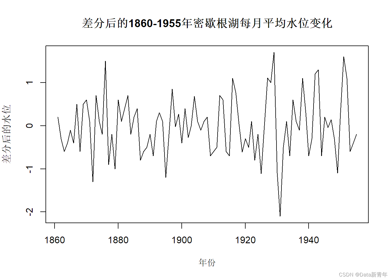
3. Perform the first-order difference operation and perform the stationarity test again:
diff_le <- diff(level)
#可视化
plot(diff_le, type = "l", main = "差分后的1860-1955年密歇根湖每月平均水位变化",
     xlab = "年份", ylab = "差分后的水位")
#进行ADF检验
adf.test(diff_le)
## Warning in adf.test(diff_le): p-value smaller than printed p-value
##
##  Augmented Dickey-Fuller Test
##
## data:  diff_le
## Dickey-Fuller = -5.6057, Lag order = 4, p-value = 0.01
## alternative hypothesis: stationary
#进行KPSS检验
kpss.test(diff_le)
## Warning in kpss.test(diff_le): p-value greater than printed p-value
##
##  KPSS Test for Level Stationarity
##
## data:  diff_le
## KPSS Level = 0.07181, Truncation lag parameter = 3, p-value = 0.1
Conclusion:
The sequence is significantly stationary after the first difference;
the p value of the KPSS test is greater than 0.05, and the null hypothesis cannot be rejected, that is, the sequence tends to be stationary under the first difference.
4. Perform ACF and PACF analysis on the first-differenced sequence to determine the ARMA model:
#ACF和PACF
par(mfrow = c(1,2))
acf(diff_le, main = "ACF")
pacf(diff_le, main = "PACF")
By performing ACF and PACF analysis on the sequence after first difference.
The ACF plot slowly decays from lags=1, indicating that an AR(1) model may be suitable for this sequence. But as the lag gets larger, the ACF gets closer and closer to 0, which means that a MA(1) model may also be suitable.
The PACF plot is censored at lags=1, indicating that an AR(1) model may be suitable. However, at lags=2, PACF is significantly negative again, which indicates that an MA(1) term may be needed to explain the sequence.
It can be seen that the ARMA(1,1) model may be a more suitable model feature.